Dualities
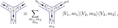
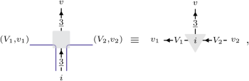
We explain here how to obtain the models dual to equation (1) considered in the main text. We encourage the reader to consult ref. 48 for further details. First, it is crucial to rewrite the local operators entering the definition of the Hamiltonian of equation (1) in such a way that the symmetry \({{\mathbb{A}}}_{4}\) is manifest. Invoking a finite group version of the Wigner–Eckart theorem, we know that any operator transforming trivially under \({{\mathbb{A}}}_{4}\) must be expressible as a linear combination of Clebsch–Gordan coefficients. The group \({{\mathbb{A}}}_{4}\) possesses three one-dimensional irreducible representations \(\{\underline{0},\underline{1},{\underline{1}}^{* }\}\) and a single three-dimensional one \(\underline{3}\) satisfying \(\underline{3}\otimes \underline{3}\cong \underline{0}\oplus \underline{1}\oplus {\underline{1}}^{* }\oplus \underline{3} \oplus \underline{3}\). Given three irreducible representations V1, V2 and V3 such that V3 ⊂ V1 ⊗ V2, we interpret the intertwining map V3 → V1 ⊗ V2 as the tensor
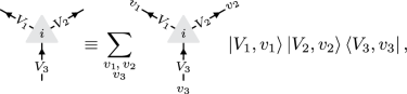
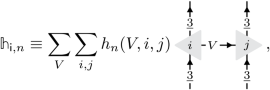
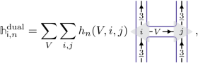
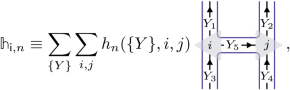
where the sums are over basis vectors and i enumerates the different ways V1 ⊗ V2 decomposes into V3. In this equation, the diagram on the right-hand side depicts the Clebsch–Gordan coefficients valued in \({\mathbb{C}}\). In this notation, we can show that the local operators \({{\mathbb{h}}}_{{\mathsf{i}},n}\), n ∈ {0, 1, 2}, are all of the form
(3)
where \({h}_{n}(V,i,j)\in {\mathbb{C}}\). Notice that in this formulation, the state space of a given spin-1 degree of freedom is spanned by \(\left\vert \underline{3},v\right\rangle\), with v = 1, …, 3.
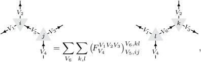
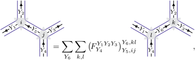
Importantly, we have the following equality of intertwining maps V4 → V1 ⊗ V2 ⊗ V3:
(2)
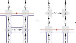
where the F symbols \({\left({F}_{{V}_{4}}^{{V}_{1}{V}_{2}{V}_{3}}\right)}_{{V}_{5},ij}^{{V}_{6},kl}\in {\mathbb{C}}\) are provided by the Racah W coefficients of \({{\mathbb{A}}}_{4}\). One can use this identity to show that the structure constants of the algebra generated by the local symmetric operators \({\{{{\mathbb{h}}}_{{\mathsf{i}},n}\}}_{{\mathsf{i}},n}\) depend only on the F symbols and coefficients \({\{{h}_{n}\}}_{n}\). Interpreting equation (4) as a tensor network equation, one can ask the following question: Is there another set of tensors, generically depicted as
(5)
(6)
also indexed by triplets of representations {V1, V2, V3 ⊂ V1 ⊗ V2} and satisfying equation (4)? Keeping \({\{{h}_{n}\}}_{n}\) the same, then replacing the intertwining maps in equation (3) by these new tensors would result in an isomorphic algebra of local operators and, thus, a dual model with Hamiltonian34which can be checked to have the same spectrum47. When dealing with a symmetry \({{\mathbb{A}}}_{4}\), one can find collections of tensors of the form of equation (5) satisfying equation (4) for any \(H\subseteq {{\mathbb{A}}}_{4}\) and [ψ] ∈ H2(H, U(1)) (ref. 69). This is because dualities correspond to (twisted) gauging maps of the symmetry \({{\mathbb{A}}}_{4}\), and there are as many ways to gauge a symmetry as there are ways to spontaneously break it. Typically, the dual Hamiltonian acts on a distinct microscopic Hilbert space, which is not necessarily a tensor product space as suggested by the graphical notation. This is consistent with the gauging interpretation, leading to theories with gauge degrees of freedom that satisfy local Gauss constraints. Given a pair (H, [ψ]), the degrees of freedom of the resulting dual model are associated with irreducible ψ-projective representations34, and as such, we label the model by \({{\mathsf{Rep}}}^{\psi }(H)\). Instead of Clebsch–Gordan coefficients, the tensors are found to evaluate to Racah W coefficients involving linear representations of G and ψ-projective representations of the subgroup H. Crucially, the initial Hamiltonian can be transmuted into any of its duals through an MPO47:
(7)
which is true for any V, i and j.
Generalized DMRG
To compute the ground states of the various models in the main text, we implemented a version of the two-site DMRG algorithm for finite chains with open boundary conditions70. The DMRG algorithm is a variational algorithm within the subspace of MPSs, which we recall is a class of wavefunctions that implement the area law of gapped phases at the microscopic level, thereby specifically targeting the physical corner of the total Hilbert space. Briefly, the DMRG algorithm proceeds as follows. Because the wavefunction is a multilinear function of the variables in all local tensors, the global optimization problem can iteratively be solved using an alternating least-squares approach71. The two-site version proceeds by blocking two sites together before solving the combined least-squares problem and finally using a singular value decomposition to split the two-site tensor into two one-site tensors. This two-site version is typically preferred, as it allows for an easier redistribution of Schmidt coefficients in the different tensor blocks.
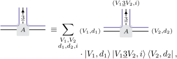
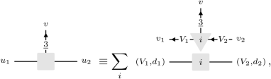
Typically, MPSs are taken to span a subspace of a tensor product space. However, an important feature of the models we consider is that they are typically not defined on a tensor product space. Rather, states need to satisfy some local kinematical constraints; these are the local Gauss constraints mentioned above. Thus, we require MPSs that explicitly enforce these kinematical constraints. For our illustrative example, this is accomplished by considering tensors of the form
(8)
where V1 and V2 are summed over ψ-projective irreducible representations of some subgroup \(H\subseteq {{\mathbb{A}}}_{4}\), i over basis vectors in the space of intertwining maps \({V}_{1}\otimes \underline{3}\to {V}_{2}\), and d1 and d2 label the remaining variational degrees of freedom. Notice that both entanglement degrees of freedom labelled by (V, d) and physical degrees of freedom labelled by \(({V}_{1}\underline{3}{V}_{2},i)\) carry gauge degrees of freedom represented by blue lines, which are shared by neighbouring physical degrees of freedom, as indicated by our graphical notation. For instance, the local Hilbert space on two sites is spanned by vectors of the form \(\left\vert {V}_{1}\underline{3}{V}_{2},i\right\rangle \left\vert {V}_{2}\underline{3}{V}_{3},j\right\rangle\). Typically, the dimension of the space of intertwining maps \({V}_{1}\otimes \underline{3}\to {V}_{2}\) depends on (V1, V2), which is incompatible with a tensor product Hilbert space. By construction, the action of the Hamiltonian of equation (6) leaves the constrained Hilbert space invariant and, thus, explicitly preserves the structure of such an MPS.
Our algorithm proceeds like the standard two-site DMRG, but all the basic operations are tailored to preserve the kinematical constraints, which amounts to maintaining the structure displayed in equation (8). First, by using block-diagonal basis transformations on the entanglement space, any MPS of the form of equation (8) can be brought into the left canonical form defined by the condition:
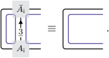
(9)
In left canonical form, the Schmidt values λ of the reduced density matrix obtained by tracing out all the sites to the right of the site \({\mathsf{i}}\) are then given by the spectrum of \({\rho }_{{\mathsf{i}}}\) defined as
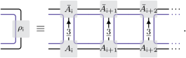
(10)
These density matrices are block diagonal, with blocks labelled by ψ-projective irreducible representations of the subgroup H. As reviewed above, a crucial step of the two-site DMRG algorithm amounts to decomposing the two-site MPS tensor that solves the combined least-squares problem into single-site MPS tensors A. Specifically, consider a tensor whose entries are of the form
(11)
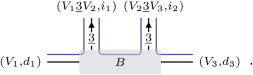
Keeping the gauge degree of freedom V2 fixed, one considers the matrix \({B}^{{V}_{2}}\) with entries
$${[{B}^{{V}_{2}}]}_{({V}_{1},{d}_{1}{i}_{1})}^{({V}_{3},{d}_{3}{i}_{2})}:={[{B}^{({V}_{1}\underline{3}{V}_{2},{i}_{1})({V}_{2}\underline{3}{V}_{3},{i}_{2})}]}_{({V}_{1},{d}_{1})}^{({V}_{3},{d}_{3})}.$$
(12)
Performing a singular value decomposition yields a factorization of the form \({B}^{{V}_{2}}={M}^{{V}_{2}}{\Sigma }^{{V}_{2}}{({N}^{{V}_{2}})}^{\dagger }\), where M and N are unitary matrices and \({\Sigma }^{{V}_{2}}\) is a diagonal matrix. The entries of Σ are all positive and are referred to as the singular values of \({B}^{{V}_{2}}\). Truncating the singular values to the desired precision λmin yields the low-rank approximation
$${[{B}^{{V}_{2}}]}_{({V}_{1},{d}_{1}{i}_{1})}^{({V}_{3},{d}_{3}{i}_{2})}\approx\sum_{k=1}^{{\lambda }_{\min }}{[{M}^{{V}_{2}}]}_{({V}_{1},{d}_{1}{i}_{1})}^{k}\,{[{\Sigma }^{{V}_{2}}]}_{k}^{k}\,{{[{N}^{{V}_{2}}]}_{({V}_{3},{d}_{3}{i}_{2})}^{k}}^{* }.$$
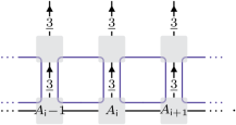
Repeating this operation for all ψ-projective representations V2 of A, one finally defines MPS tensors \({A}_{{\mathsf{i}}}\) and \({A}_{{\mathsf{i}}+1}\):
$$\begin{aligned}{[{A}_{{\mathsf{i}}}^{({V}_{1}\underline{3}{V}_{2},{i}_{1})}]}_{({V}_{1},{d}_{1})}^{({V}_{2},k)}&:={[{M}^{{V}_{2}}]}_{({V}_{1},{d}_{1}{i}_{1})}^{k}\\ \text{and}\quad {[{A}_{{\mathsf{i}}+1}^{({V}_{2}\underline{3}{V}_{3},{i}_{2})}]}_{({V}_{2},k)}^{({V}_{3},{d}_{3})}&:={[{\Sigma }^{{V}_{2}}]}_{k}^{k}\,{{[{N}^{{V}_{2}}]}_{({V}_{3},{d}_{3}{i}_{2})}^{k}}^{* },\end{aligned}$$
(13)
respectively, so that equation (11) is approximated by
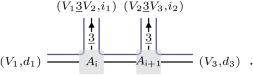
(14)
We can then repeat the same steps for the sites \({\mathsf{i}}+1\) and \({\mathsf{i}}+2\) and keep on sweeping from left to right and then from right to left.
In our simulations, we initialized the bulk of the MPS with random matrices of a given dimension per block V2, whereas on the boundary, we imposed a restriction to a single one-dimensional block. This corresponds to a choice of boundary condition for the MPO transmuting the Hamiltonian of the model that we are simulating into the initial one. In the very specific cases where our algorithm is equivalent to the standard symmetry-preserving DMRG, this amounts to the customary fixing of the total charge sector of the state. Finally, note that our approach is not specific to the two-site DMRG. In particular, uniform MPS algorithms for infinite chains (including variational uniform MPS (VUMPS) and ‘pulling-through’ algorithms) can also be implemented72,73.
Symmetries in tensor networks
Next, we clarify the specific scenarios in which our algorithm amounts to using symmetry-preserving tensors. Consider a Hamiltonian with an ordinary symmetry encoded into a (finite) group G. Suppose the Hamiltonian is in the G symmetric phase. We claim that the optimal way of simulating this phase through the DMRG algorithm is to simulate the dual model obtained by gauging G, before acting with the MPO transmuting the Hamiltonian of the dual model into the initial one. Within our framework, gauging G means that we are dealing with MPS tensors of the form of equation (8), where the gauge degrees of freedom depicted by the blue lines are also labelled by irreducible representations of G. The building blocks of the MPO for this duality then evaluate to Clebsch–Gordan coefficients. More precisely, for the model in equation (3), where the local Hilbert space is spanned by \(\left\vert \underline{3},v\right\rangle\), v = 1, …, 3, we have the following identification:
(15)
whereby the MPO tensor acts on the space of intertwining maps \({V}_{1}\otimes \underline{3}\to {V}_{2}\). Acting with this MPO then yields an MPS of the form:
(16)
We show that, in this very specific case, our procedure amounts to directly simulating the initial phase using symmetry-preserving tensor networks49,50,51. Generally, symmetry-preserving tensor network algorithms exploit a specific expression for the tensors that explicitly enforces the symmetry. Concretely, consider an MPS in the Hilbert space of the model of equation (6). Generically, entanglement degrees of freedom of the MPS tensor live in a vector space U. Let us suppose that the MPS tensors are invariant under the action of \({{\mathbb{A}}}_{4}\). As already exploited, the Wigner–Eckart theorem stipulates that the tensors are expressible as linear combination of Clebsch–Gordan coefficients. More concretely, because the vector space U is equipped with an \({{\mathbb{A}}}_{4}\) action, it can be decomposed into irreducible representations, that is U ≅ ⨁V〈U, V〉V, where the direct sum is over irreducible representations of \({{\mathbb{A}}}_{4}\) and \(\langle V,U\rangle \in {{\mathbb{Z}}}_{\ge 0}\). It follows that we can decompose u = 1, …, dim U as (V, v, d) ≡ (V, v) ⊗ (V, d), where v = 1, …, dim V and d = 1, …, 〈U, V〉. Using this notation, the MPS tensors decompose as follows:
(17)
revealing in particular the sparse block structure of the tensors. As per our graphical calculus, the matrices on the right-hand side labelled by i are, in fact, of the form of equation (8). From a symmetric tensor network viewpoint, this decomposition is used to target a specific charge sector of the Hilbert space, thereby reducing computational costs while explicitly enforcing the symmetry49,50,51. Let us now assume that the MPS is the unique ground state of the \({{\mathbb{A}}}_{4}\) symmetric phase. In this case, equation (17) precisely recovers equation (16) under the identification of equation (15) such that the entanglement degrees of freedom of the MPS ground state of the dual model are labelled by pairs (V, d). One can now verify that our algorithm then produces a result that agrees with symmetry-preserving DMRG. However, on comparing our algorithm to current state-of-the-art implementations, our approach is practically much simpler because it does not require the conventional implementation of the recoupling theory for symmetric tensors based on fusion trees.
As commented in the main text, this decomposition is tailored to the symmetric phase for which entanglement degrees of freedom of the unique ground state transform as linear representations of \({{\mathbb{A}}}_{4}\). By contrast, this is clearly not suited to the \({{\mathbb{A}}}_{4}\) SPT phase, for which entanglement degrees of freedom transform as projective representations of \({{\mathbb{A}}}_{4}\). Indeed, it is well known that using standard symmetric tensor networks in an SPT phase is more costly because it forces the edge modes to transform according to a linear representation, which requires further long-range entanglement74.
In practice, most of the utility of symmetry-preserving tensor networks is in models with continuous Lie group symmetries, such as SU(2). Although we restricted ourselves to a finite group, our results readily generalize to these cases, implying, for instance, that a ground state preserving an SU(2) symmetry is most efficiently described in terms of the ground state of a dual model that breaks a dual non-invertible \({\mathsf{Rep}}({\text{SU}}(2))\) symmetry. For this case, the duality transformation recovers the celebrated Schur–Weyl duality. The resulting dual models are the so-called interaction-round-a-face models studied by Sierra and Nishino61. Because the different symmetry-broken ground states are related by the action of non-trivial symmetry MPOs, these ground states do not have the same entanglement, which shows the importance of properly initializing the DMRG algorithm to favour the ground states with the least amount of entanglement. Note that the fact that SU(2) admits an infinite number of irreducible representations is practically addressed by assigning a weight zero to higher spin ones, so that we effectively deal with a finite number of blocks only, just as in standard DMRG exploiting symmetry-preserving tensors.
Mathematical formalism
We summarize here the mathematical formalism underpinning the results presented in the main text. More precise mathematical definitions can be found, for instance, in ref. 29. Consider any local one-dimensional quantum lattice model with a generalized symmetry encoded into a fusion category \({\mathcal{C}}\). In the presence of such a generalized symmetry, gapped phases are characterized by a choice of an (indecomposable) \({\mathcal{C}}\)-module category, whose objects label the degenerate ground states of the phase23,36. The same module categories also characterize the different ways to gauge (sub)symmetries of the model. After performing the gauging operation associated with a \({\mathcal{C}}\)-module category \({\mathcal{M}}\), the dual symmetry of the resulting model is encoded into the so-called Morita dual \({{\mathcal{C}}}_{{\mathcal{M}}}^{* }\) of \({\mathcal{C}}\) with respect to \({\mathcal{M}}\). The fusion category \({{\mathcal{C}}}_{{\mathcal{M}}}^{* }\) is defined to be the category \({{\mathsf{Fun}}}_{{\mathcal{C}}}({\mathcal{M}},{\mathcal{M}})\) of \({\mathcal{C}}\)-module endofunctors of \({\mathcal{M}}\) (refs. 29,75), the fusion structure being provided by the composition of \({\mathcal{C}}\)-module functors. Crucially, \({\mathcal{M}}\) is also a \({{\mathcal{C}}}_{{\mathcal{M}}}^{* }\)-module category, and we have \({({{\mathcal{C}}}_{{\mathcal{M}}}^{* })}_{{\mathcal{M}}}^{* }\simeq {\mathcal{C}}\). In other words, there is always a way to gauge a subsymmetry of \({{\mathcal{C}}}_{{\mathcal{M}}}^{* }\) so as to recover the initial model.
Let us examine this gauging operation in practice. For conciseness, we focus on nearest-neighbour Hamiltonians, but longer-range interactions can be accommodated just as easily. As for the example studied in the main text, it is crucial to write the Hamiltonian in such a way that the generalized symmetry \({\mathcal{C}}\) is manifest. Under some mild mathematical assumptions about the symmetry MPOs32,76, it follows from a generalized Wigner–Eckart theorem33 that any local symmetric operator is expressible in terms of generalized Clebsch–Gordan coefficients. Specifically, given a \({\mathcal{C}}\)-symmetric Hamiltonian of the form \({\mathbb{H}}=\sum_{{\mathsf{i}} = 1}^{L-1}\sum_{n}{{\mathbb{h}}}_{{\mathsf{i}},n}\), the local operators can always be put in the form
(18)
in terms of tensors evaluating to these generalized Clebsch–Gordan coefficients. The graphical notation mimics that of equation (6) and encodes, in particular, that the Hilbert space of a model with a generalized symmetry is generically not a tensor product space. More concretely, there is a (possibly not unique) choice of \({\mathcal{C}}\)-module category \({\mathcal{R}}\) such that local operators can be expressed as equation (18), where {Y} label objects in \({{\mathcal{C}}}_{{\mathcal{R}}}^{* }\), and the generalized Clebsch–Gordan coefficients are given by the so-called module associator of \({\mathcal{R}}\), as a \({{\mathcal{C}}}_{{\mathcal{R}}}^{* }\)-module category (see refs. 32,34,47 for details).
It follows from the defining axioms of the \({{\mathcal{C}}}_{{\mathcal{R}}}^{* }\)-module category \({\mathcal{R}}\) that the tensors in equation (18) satisfy an analogue of equation (4):
(19)
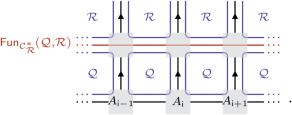
where the F symbols \({\left({F}_{{Y}_{4}}^{{Y}_{1}{Y}_{2}{Y}_{3}}\right)}_{{Y}_{5},ij}^{{Y}_{6},kl}\in {\mathbb{C}}\) enter the definition of the fusion category \({{\mathcal{C}}}_{{\mathcal{R}}}^{* }\). Together with the complex coefficients {hn}n, these F symbols provide the structure constants of the algebra generated by the local symmetric operators \({\{{{\mathbb{h}}}_{{\mathsf{i}},n}\}}_{{\mathsf{i}},n}\). Within this framework, performing a gauging operation simply amounts to picking a different \({{\mathcal{C}}}_{{\mathcal{R}}}^{* }\)-module category \({{\mathcal{R}}}^{{\prime} }\). This means replacing the tensors in equation (18) by a new set of tensors that now evaluate to generalized Clebsch–Gordan coefficients given by the module associator of \({{\mathcal{R}}}^{{\prime} }\). Crucially, this new set of tensors still satisfy equation (19), so the algebra of local symmetric operators generated by equation (18) is isomorphic to the initial one. The dual symmetry of the resulting model is then encoded into the fusion category \({({{\mathcal{C}}}_{{\mathcal{R}}}^{* })}_{{{\mathcal{R}}}^{{\prime} }}^{* }\). Like the examples discussed in the main text, Hamiltonians associated with different choices of \({{\mathcal{C}}}_{{\mathcal{R}}}^{* }\)-module categories can be transmuted into each other through an MPO. Mathematically, such an operator is described by an object in the category \({{\mathsf{Fun}}}_{{{\mathcal{C}}}_{{\mathcal{R}}}^{* }}({\mathcal{R}},{{\mathcal{R}}}^{{\prime} })\) of \({{\mathcal{C}}}_{{\mathcal{R}}}^{* }\)-module functors from \({\mathcal{R}}\) to \({{\mathcal{R}}}^{{\prime} }\), in such a way that the building blocks of the MPO are provided by the module structure of such a functor47. Moreover, this category of module functors has the structure of a module category \({\mathcal{M}}\) over the symmetry category \({\mathcal{C}}\simeq {{\mathsf{Fun}}}_{{{\mathcal{C}}}_{{\mathcal{R}}}^{* }}({\mathcal{R}},{\mathcal{R}})\) through composition of module functors. We identify this \({\mathcal{C}}\)-module category as that encoding the gauging operation corresponding to changing the \({{\mathcal{C}}}_{{\mathcal{R}}}^{* }\)-module category \({\mathcal{R}}\) into \({{\mathcal{R}}}^{{\prime} }\) in such a way that the dual symmetry is encoded into \({{\mathcal{C}}}_{{\mathcal{M}}}^{* }\simeq {({{\mathcal{C}}}_{{\mathcal{R}}}^{* })}_{{{\mathcal{R}}}^{{\prime} }}^{* }\). Note that for many fusion categories of interest, indecomposable module categories have been classified. Importantly, the data of the module functors needed to describe the MPO intertwiners relating the different dual models can be obtained as a representation theoretic problem33,77, which numerically can be reduced to a linear algebra problem.
Let us now suppose that the initial \({\mathcal{C}}\)-symmetric model, which is defined with respect to the \({{\mathcal{C}}}_{{\mathcal{R}}}^{* }\)-module category \({\mathcal{R}}\), is in the phase associated with the \({\mathcal{C}}\)-module category \({\mathcal{P}}\). Our goal is to find a dual model whose dual symmetry is completely broken in the ground-state subspace. To achieve this, we must understand how to relate the phase of the dual model to the phase of the initial model, which is not immediate given that the symmetry structures differ. To this end, we can think of the \({\mathcal{C}}\)-module category \({\mathcal{P}}\) as \({{\mathsf{Fun}}}_{{{\mathcal{C}}}_{{\mathcal{R}}}^{* }}({\mathcal{R}},{\mathcal{Q}})\) for some \({{\mathcal{C}}}_{{\mathcal{R}}}^{* }\)-module category \({\mathcal{Q}}\). Indeed, because \({\mathcal{C}}\simeq {{\mathsf{Fun}}}_{{{\mathcal{C}}}_{{\mathcal{R}}}^{* }}({\mathcal{R}},{\mathcal{R}})\), it does define a \({\mathcal{C}}\)-module category through composition of module functors. Because any \({\mathcal{C}}\)-module category can be constructed in this way29, it follows that \({\mathcal{P}}\) uniquely fixes \({\mathcal{Q}}\). The action of a duality operator \({{\mathsf{Fun}}}_{{{\mathcal{C}}}_{{\mathcal{R}}}^{* }}({\mathcal{R}},{{\mathcal{R}}}^{{\prime} })\) on the phase \({\mathcal{P}}\) can now be obtained through composition of module functors, such that the new phase is encoded into \({{\mathsf{Fun}}}_{{{\mathcal{C}}}_{{\mathcal{R}}}^{* }}({{\mathcal{R}}}^{{\prime} },{\mathcal{Q}})\), which is indeed a module category over the dual symmetry \({({{\mathcal{C}}}_{{\mathcal{R}}}^{* })}_{{{\mathcal{R}}}^{{\prime} }}^{* }={{\mathsf{Fun}}}_{{{\mathcal{C}}}_{{\mathcal{R}}}^{* }}({{\mathcal{R}}}^{{\prime} },{{\mathcal{R}}}^{{\prime} })\). The optimal dual model, whose dual symmetry is completely broken, is obtained when the module category that describes the dual phase is given by the dual symmetry itself. From the above, it is clear that this amounts to choosing \({{\mathcal{R}}}^{{\prime} }={\mathcal{Q}}\) so that \({\mathcal{Q}}\) encodes the degrees of freedom. Consider a variational ground-state MPS in the constrained Hilbert space of the optimal dual model with degrees of freedom in \({\mathcal{Q}}\), which maximally breaks the dual symmetry. The remaining symmetry-breaking ground states can be obtained by acting with symmetry MPOs labelled by simple objects in \({{\mathcal{C}}}_{{\mathcal{P}}}^{* }\) of the form
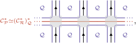
(20)
where the individual tensors are determined by the data of the relevant \({{\mathcal{C}}}_{{\mathcal{R}}}^{* }\)-module functors47. Finally, these dual ground states can be mapped to ground states of the original model, which is defined with respect to the \({{\mathcal{C}}}_{{\mathcal{R}}}^{* }\)-module category \({\mathcal{R}}\), by acting with a duality MPO:
(21)
Conversely, the duality operators in the optimal model are encoded into \({{\mathsf{Fun}}}_{{{\mathcal{C}}}_{{\mathcal{R}}}^{* }}({\mathcal{R}},{\mathcal{Q}})\), which is equivalent to the \({\mathcal{C}}\)-module category \({\mathcal{P}}\) encoding the phase of the original model. The various fusion categories and the Morita equivalences between them, both before and after the duality, can be summarized as
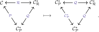
(22)
To conclude, we revisit our example in light of this general formalism. When dealing with an ordinary (invertible) symmetry \({{\mathbb{A}}}_{4}\), the corresponding fusion category \({\mathcal{C}}\) is the category \({{\mathsf{Vec}}}_{{{\mathbb{A}}}_{4}}\) of \({{\mathbb{A}}}_{4}\)-graded vector spaces. The different ways to gauge subsymmetries of \({{\mathbb{A}}}_{4}\) are provided by \({{\mathsf{Vec}}}_{{{\mathbb{A}}}_{4}}\)-module categories, which are known to be classified by pairs (A, [ψ]), as defined in the main text69. In particular, choosing A = G and ψ = 1 amounts to the (untwisted) gauging of A, and the corresponding \({{\mathsf{Vec}}}_{{{\mathbb{A}}}_{4}}\)-module category is equivalent to the category \({\mathsf{Vec}}\) of complex vector spaces. The Morita dual \({({{\mathsf{Vec}}}_{{{\mathbb{A}}}_{4}})}_{{\mathsf{Vec}}}^{* }\) of \({{\mathsf{Vec}}}_{{{\mathbb{A}}}_{4}}\) with respect to \({\mathsf{Vec}}\) can be confirmed to be equivalent to the category \({\mathsf{Rep}}({{\mathbb{A}}}_{4})\) of representations of \({{\mathbb{A}}}_{4}\), in agreement with our results. When writing the Hamiltonian as in equation (1), we are choosing the \({\mathsf{Rep}}({{\mathbb{A}}}_{4})\)-module category \({\mathcal{R}}={\mathsf{Vec}}\) such that the module associator boils down to the ordinary Clebsch–Gordan coefficients of \({{\mathbb{A}}}_{4}\). We obtain the various dual models by choosing different \({\mathsf{Rep}}({{\mathbb{A}}}_{4})\)-module categories. Specifically, the dual model resulting from the ψ-twisted gauging of H is obtained by choosing the module category \({{\mathcal{R}}}^{{\prime} }={{\mathsf{Rep}}}^{\psi }(H)\) of ψ-projective representations of H, and the dual symmetry is encoded into \({({\mathsf{Rep}}({{\mathbb{A}}}_{4}))}_{{{\mathsf{Rep}}}^{\psi }(H)}^{* }\).
We now suppose that the initial model is in the phase associated with the \({{\mathsf{Vec}}}_{{{\mathbb{A}}}_{4}}\)-module category \({\mathcal{M}}(K,\phi ):={{\mathsf{Fun}}}_{{\mathsf{Rep}}({{\mathbb{A}}}_{4})}({\mathsf{Vec}},{{\mathsf{Rep}}}^{\phi }(K))\). The \({{\mathbb{A}}}_{4}\) SPT, \({{\mathbb{A}}}_{4}\) symmetric and \({{\mathbb{D}}}_{2}\) symmetric phases considered in the main text were obtained by choosing \({{\mathsf{Rep}}}^{\phi }(K)\) to be equal to \({{\mathsf{Rep}}}^{\psi }({{\mathbb{A}}}_{4})\), \({\mathsf{Rep}}({{\mathbb{A}}}_{4})\) and \({\mathsf{Rep}}({{\mathbb{D}}}_{2})\), respectively. The optimal model is always found to be that given by \({{\mathcal{R}}}^{{\prime} }={{\mathsf{Rep}}}^{\phi }(K)\), which amounts to performing a ϕ-twisted gauging of K, as predicted. The relevant Morita equivalences can be summarized as
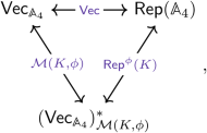
(23)
where the phase is encoded in the \({{\mathsf{Vec}}}_{{{\mathbb{A}}}_{4}}\)-module category \({\mathcal{M}}(K,\phi )\), which states that the different ground states are labelled by cosets in G/K and the remaining symmetry K acts ϕ-projectively.
Let us also shed light on some of the suboptimal simulations. For instance, consider the \({{\mathbb{A}}}_{4}\)-symmetric phase and the dual model labelled by \({{\mathcal{R}}}^{{\prime} }={{\mathsf{Rep}}}^{\psi }({{\mathbb{D}}}_{2})\). The symmetry is \({({\mathsf{Rep}}({{\mathbb{A}}}_{4}))}_{{{\mathsf{Rep}}}^{\psi }({{\mathbb{D}}}_{2})}^{* }\simeq {{\mathsf{Vec}}}_{{{\mathbb{A}}}_{4}}\), whereas the dual phase is that associated with the \({{\mathsf{Vec}}}_{{{\mathbb{A}}}_{4}}\)-module category \({{\mathsf{Fun}}}_{{\mathsf{Rep}}({{\mathbb{A}}}_{4})}({{\mathsf{Rep}}}^{\psi }({{\mathbb{D}}}_{2}),{\mathsf{Rep}}({{\mathbb{A}}}_{4}))\simeq {\mathsf{Vec}}\). Moreover, because \({{\mathsf{Rep}}}^{\psi }({{\mathbb{D}}}_{2})\) is equivalent to \({\mathsf{Vec}}\) as a category, this explains why the numerical results were the same for this dual model as for the initial one. In a similar vein, in the \({{\mathbb{A}}}_{4}\) SPT phase, the dual model obtained by choosing \({{\mathcal{R}}}^{{\prime} }={\mathsf{Rep}}({{\mathbb{D}}}_{2})\) has a \({({\mathsf{Rep}}({{\mathbb{A}}}_{4}))}_{{\mathsf{Rep}}({{\mathbb{D}}}_{2})}^{* }\simeq {{\mathsf{Vec}}}_{{{\mathbb{A}}}_{4}}\) symmetry. The dual phase is associated with the \({{\mathsf{Vec}}}_{{{\mathbb{A}}}_{4}}\)-module category \({{\mathsf{Fun}}}_{{\mathsf{Rep}}({{\mathbb{A}}}_{4})}({\mathsf{Rep}}({{\mathbb{D}}}_{2}),{{\mathsf{Rep}}}^{\psi }({{\mathbb{A}}}_{4}))\), which is equivalent to \({\mathsf{Vec}}\) as a category, meaning that the whole symmetry is preserved, in agreement with our numerical results. Finally, let us examine the \({{\mathbb{D}}}_{2}\) symmetric phase and the dual model obtained by choosing the \({{\mathsf{Vec}}}_{{{\mathbb{A}}}_{4}}\)-module category \({{\mathcal{R}}}^{{\prime} }={\mathsf{Rep}}({{\mathbb{Z}}}_{3})\). The dual symmetry \({({\mathsf{Rep}}({{\mathbb{A}}}_{4}))}_{{\mathsf{Rep}}({{\mathbb{Z}}}_{3})}^{* }\simeq {\mathsf{Rep}}({{\mathbb{A}}}_{4})\) is also fully preserved because the module category over it is \({{\mathsf{Fun}}}_{{\mathsf{Rep}}({{\mathbb{A}}}_{4})}({\mathsf{Rep}}({{\mathbb{Z}}}_{3}),{\mathsf{Rep}}({{\mathbb{D}}}_{2}))\), which happens to be equivalent to \({\mathsf{Vec}}\), in agreement with our numerical results.