This study was conducted in accordance with the Declaration of Helsinki and received approval from the ethics committee of Rambam Health Care Campus, which waived the requirement for a consent form. The Helsinki approval number is RMB-D-0653-21.
Data
Our dataset is derived from patient records encompassing the period from 2010 to 2022 at a pediatric ophthalmology clinic. Each record in the dataset corresponds to a patient’s visit, providing essential details such as a unique patient identifier, visit date, patient age at the time of the visit, obstetric history, family history of ophthalmological conditions, medical history, and comprehensive information gathered during the visit. Notably, in the current study, we did not utilize the textual information describing family history, medical history, or obstetric history. Instead, we introduced corresponding binary variables indicating whether these fields held the default value, signifying evidence for a problem or not. This approach allows us to incorporate relevant information while simplifying the analysis by converting textual data into a more structured and analytically accessible format. The list of variables, their descriptions and descriptive statistics are shown in Table 1 in the Results section.
A patient is classified as having myopia, or a myopic refractive error, if the spherical equivalent in either the left or right eye is ≤ − 0.50 D. The spherical equivalent is computed from the sphere and astigmatism obtained after the administration of cyclopentolate 1% drops for each eye, according to the formula:
\(spherical{\text{ }}equivalent\,=\,objective{\text{ }}refraction{\text{ }}sphere\,+\,0.5 \times objective{\text{ }}refraction{\text{ }}astigmatism\)
While the conventional definition of myopia onset typically requires a spherical equivalent of − 0.50 D or more in both eyes, our study focuses on detecting the earliest signs of myopic progression in a previously non-myopic population. To capture these subtle changes, we classified myopia even if it was identified in only one eye.
The dataset comprises a total of 15,162 visits from 7937 patients. In our pursuit of predicting myopia, we excluded patients with only one clinic visit and those who presented with myopia during their initial visit. In other words, we included only patients who had at least two visits and were not diagnosed with myopia in their first visit. This resulted in a refined dataset consisting of 7814 visits involving 2437 patients. Among this cohort, 429 (11%) individuals eventually developed myopia. The mean follow-up duration per patient was 3.08 years.
Data preparation
In cases where variables such as objective refraction sphere, cylinder, and angle had missing values, typically due to non-measurement during a particular visit by the physician, we addressed this by imputing the missing values from the preceding visit of that specific patient, and only in cases where the preceding visit occurred within a short time frame, usually within three months, ensuring the substituted data remained clinically valid and temporally consistent. This approach allowed us to retain as much of the dataset as possible, minimizing the loss of potentially valuable information while maintaining the continuity of individual patient data across visits.
We introduced three additional variables for each visit, serving as target variables for the prediction models detailed below:
-
(1)
Is myopia last: Indicates whether the patient developed myopic refractive change at some point after the visit.
-
(2)
Is myopia next: Indicates whether new myopic refractive error was detected at the patient’s subsequent visit.
-
(3)
Is myopia within year: Indicates whether any myopic refractive change occurred within one year of the visit.
These variables reflect the future trajectory of the patient based on their follow-up visits. Consider, for example, a patient who is not myopic at Visit 1 but later develops myopia at Visit 4. This patient would be categorized in the first visit as follows: Is myopia last = True if Visit 4 is the final recorded visit and results in a myopia diagnosis; Is myopia next = False because the next visit does not results in a myopia diagnosis; Is myopia within year = False if the time between Visit 1 and Visit 4 is more than or equal to one year.
Finally, to maintain the focus on predicting myopia, we removed all visits where patients already had myopia.
Model development
We constructed three distinct myopia prediction models:
-
Model 1
This model predicts whether a patient will develop myopia at some point based solely on their first visit. The dataset for training this model included only the first visits of patients who had at least two visits. In total there were 2437 such visits. The target variable in this model indicates whether the patient developed myopia after the first visit, with 279 (11.4%) patients eventually developing myopia.
-
Model 2
For each visit in which the patient had no myopia, this model predicts whether they will be diagnosed with myopia in the subsequent visit. Thus, the dataset for training this model included all visits of patients not diagnosed with myopia who had a subsequent visit (in total there are 5320 such visits). The target variable denoted whether the patient was diagnosed with myopia in the next visit, with a total of 317 (6%) patients receiving such a diagnosis.
-
Model 3
This model predicts, for each visit without myopia, whether the patient will be diagnosed with myopia within a year. The training dataset for this model encompassed all visits where patients were without myopia and had a subsequent visit within a year, totaling 2297 instances. The target variable indicated whether the patient was diagnosed with myopia within a year from the visit, with 172 (5.7%) visits resulting in myopia diagnoses within the specified timeframe.
Figure 1 shows the study cohort and its subsets used for each model.
In all three models the predictors that were used are: age, gender, obstetrical history, medication sensitivity, medical history, ophthalmology history, slit lamp eye examination, visual acuity, cycloplegic refraction, and amblyopia (please refer to Table 1). Please note that the following variables: obstetrical history, medication sensitivity, medical history, ophthalmology history and slit lamp eye examination are binary (0 non-existing or 1 existing). It should also be noted that although refractive error measurements from the left and right eyes are typically correlated, we chose to include both in the model based on empirical evaluation. When we tested simplified versions of the models using only the right eye’s refractive data, predictive performance consistently declined (AUC decreased by more than 0.01 across all models). Furthermore, of the 7814 visits included in our study, 1437 (18.4%) exhibited a spherical equivalent (SE) difference of ≥ 0.50 D between eyes (mean difference = 0.15 D, SD = 0.36), suggesting that interocular asymmetry may carry clinically relevant information. For these reasons, we retained refractive features from both eyes to preserve predictive signal and maintain clinical fidelity.
We trained these three models using two widely adopted machine learning classification algorithms: “Random Forest (RF)” and “Gradient Boosting Tree (GBT)”, both available in the scikit-learn Python library42. These models are popular and considered very effective for classification36,43 .
The RF classifier creates a “forest” comprised of decision trees, each trained on a randomly chosen subset of features. By harnessing the collective wisdom of these trees, the RF model makes predictions for a given sample by consolidating their individual outputs. The final classification is determined by a majority voting system, where the most commonly predicted class across the trees is chosen as the ultimate label44,45.
In contrast, the GBT classifier is also an ensemble model consisting of multiple decision trees (weak learners), combined to form a powerful predictive model. During training, trees are incrementally added to the model, with each subsequent tree aimed at reducing the model’s error through a gradient descent approach. GBT models excel in uncovering intricate patterns within data, rendering them particularly advantageous for classification tasks46.
Both models are able to uncover complex relationships between these variables and the dependent variable. In addition, they are not constrained by statistical assumptions (e.g., no multicollinearity between independent variables, independent observations, or specific relation between the dependent and independent variables).
Besides generating predictions, both of these models provide a feature-importance analysis capability47which can be used for learning about the variables mostly linked to the development of myopia. These scores provide a quantitative measure of the relative contribution of each variable to the model’s predictive performance. Higher scores indicate that the variable plays a more significant role in distinguishing between outcomes, while lower scores suggest limited or negligible influence.
We employed feature importance analysis not only to rank predictors, but also to guide a stepwise feature elimination procedure aimed at simplifying the models while preserving predictive performance. Starting with the least important feature (based on importance scores), we iteratively removed one variable at a time and re-evaluated model performance. If performance (AUC) remained stable or improved, the feature was permanently excluded. If performance degraded, the feature was reintroduced. This process continued until no further improvements could be achieved through feature removal. By using this approach, we ensured that the final models retained only the most informative features, thereby improving interpretability and reducing the risk of overfitting, while maintaining or enhancing predictive accuracy.
Fig. 1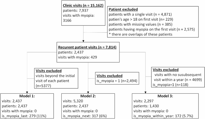
Study cohort. The figure shows how the subsets used for each model were derived.
Due to the inherent imbalance in our datasets, with the percentage of patients developing myopia significantly smaller than those who do not (11%), we address this discrepancy through up-sampling techniques, such as Synthetic Minority Over-sampling Technique (SMOTE)48. The objective of up-sampling is to generate artificial samples that mirror the characteristics of existing samples in the minority class. This approach aids the model in better learning the nuances of the minority class and enhances its predictive capabilities.
The evaluation of model performance employed standard machine learning metrics, including accuracy, sensitivity (recall), specificity, precision, F1-score (the harmonic mean of precision and recall, providing a balance between the two), and area under the receiver operating characteristic (ROC) curve (AUC). To ensure the robustness and significance of the results, a 10-fold cross-validation procedure was implemented. K-fold cross-validation is a model evaluation technique in ML where the dataset is divided into K equally sized folds, and the model is trained and tested K times, each time using a different fold as the test set and the remaining data as the training set. The performance metrics from each iteration were averaged to assess the model’s overall performance. To prevent data leakage and ensure the integrity of the cross-validation process for all models, we ensured that all visits by the same patient were exclusively present in either the training set or the test set. This precautionary measure is crucial to maintain the independence of the training and testing phases, avoiding any inadvertent sharing of information between them.