An efficient machine-learning framework for predicting protein post-translational modification sites

Hyperparameter optimization

The LightGBM classifier for Khib site prediction requires systematic hyperparameter optimization to achieve optimal predictive performance. This optimization was performed using Optuna 69, a state-of-the-art framework that employs Bayesian optimization with Tree-structured Parzen Estimators (TPE) to efficiently explore hyperparameter spaces. The optimization process was configured to maximize the AUC as the objective function, with a total of 100 trials executed to ensure a comprehensive exploration of the parameter space.

Optuna TPE algorithm iteratively refines hyperparameter selection through a probabilistic model that balances the exploration of unexplored regions with the exploitation of promising parameter combinations. This approach demonstrated convergence behaviour with optimal AUC values stabilizing after approximately 60–70 trials, indicating efficient parameter space exploration. Table 2 lists the eight main hyperparameters we focused on: number of estimators (n_estimators), learning rate, maximum tree depth, number of leaves, feature subsampling ratio (colsample_bytree), data subsampling ratio (subsample), and minimum child samples. The parameter ranges were chosen following common LightGBM best practices.

The hyperparameter optimization yielded an improvement over default LightGBM settings, with the optimized configuration achieving an AUC improvement of approximately 4.2% compared to the baseline model. Convergence analysis revealed that the optimization process efficiently identified near-optimal parameter combinations, with minimal performance variance observed in the final 20 trials, confirming the robustness of the selected hyperparameters.

Table 2 Key parameters of the LightGBM classifier and optimal settings.Comparative evaluation of feature representation methods on validation datasets

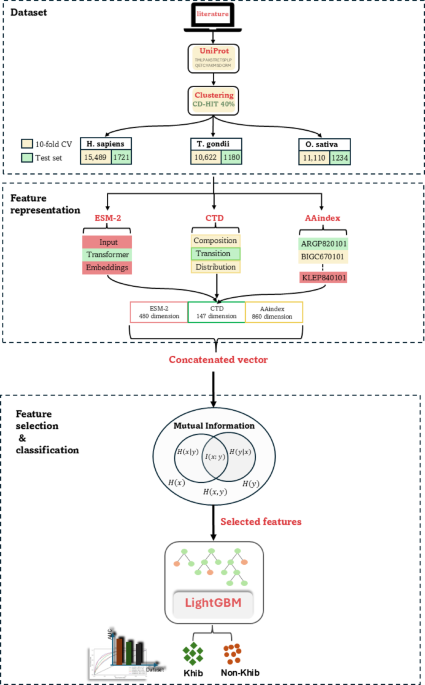
The development of an effective predictor for Khib sites using LightGBM necessitates a comprehensive evaluation of various feature representation methods to determine their discriminative capacity. This investigation comprises five distinct protein-encoding schemes that capture complementary aspects of protein sequences. The embedding-based scheme, ESM-2, leverages deep learning to extract contextual information from protein sequences. In contrast, the descriptors-based schemes, C-CTD, T-CTD, and D-CTD, encode sequence-level features that represent compositional, transitional, and distributional characteristics, respectively. The property-based scheme, AAindex, encodes intrinsic physicochemical properties of amino acids, providing insights into their biochemical attributes.

To maximize the feature space and enhance predictive performance, these encoding schemes were systematically integrated into hybrid feature sets, resulting in four additional combinations as detailed in Tables S4–S6. These combinations include: (1) CTD, which integrates C-CTD, T-CTD, and D-CTD; (2) CTD + ESM; (3) AAindex + ESM; and (4) AAindex + CTD. Additionally, a comprehensive “All Features” set was created by integrating all five individual encoding methods. Performance assessment was conducted across three species-specific datasets (H. sapiens, T. gondii, and O. sativa) using stratified 10-fold cross-validation to ensure balanced class distributions. The performance metrics revealed distinct patterns across the datasets, with notable variations in the efficacy of different feature representation methods (Tables S4–S6).

In the H. sapiens dataset (Table S4), the AAindex encoding method demonstrated excellent performance among individual representations, achieving an ACC of 0.780 and an AUC of 0.857. This performance significantly surpassed those of other individual methods (ESM, C-CTD, T-CTD, and D-CTD) by margins of 10.5% −19.82% for ACC and 10.58% −21.56% for AUC. The integration of AAindex with other encoding methods yielded statistically significant improvements. Specifically, the AAindex + CTD combination achieved an ACC of 0.790 and an AUC of 0.872, while the comprehensive “All Features” approach demonstrated the highest overall performance with an ACC of 0.791 and an AUC of 0.874. Notably, the MCC, a balanced measure of classification quality, reached 0.584 with the “All Features” approach, indicating robust discriminative capacity.

Analysis of the T. gondii dataset (Table S5) revealed that the AAindex encoding scheme again exhibited advanced performance among individual methods, with ACC and AUC values of 0.741 and 0.816, respectively. These values exceeded the average ACC and AUC of the other four individual encoding methods by 6.77% and 6.38%, respectively. Hybrid feature combinations demonstrated marked improvements, with the AAindex + CTD combination achieving an ACC of 0.764 and an AUC of 0.848. The “All Features” integration yielded the highest performance metrics (ACC of 0.766, and AUC of 0.852), ensuring that a comprehensive feature representation captures complementary aspects of the sequence information, effectively for this organism.

For the O. sativa dataset (Table S6), the individual encoding methods demonstrated moderate performance, with AAindex again outperforming other individual methods (ACC of 0.735, and AUC of 0.802). The hybrid feature combinations showed incremental enhancements, with AAindex + CTD achieving an ACC of 0.755 and an AUC of 0.834. The “All Features” integration demonstrated the highest overall performance (ACC of 0.760, and AUC of 0.838), with a notable improvement in sensitivity (SN of 0.806) compared to individual methods. The MCC value of 0.522 for the “All Features” approach indicates notable improvement over individual encoding schemes, confirming the benefits of feature integration for this organism.

To validate the robustness of our approach and ensure that the observed patterns are not model-specific, parallel experiments were performed using Random Forest (RF), XGBoost, and CatBoost classifiers, with the H. sapiens dataset serving as a representative case. The supplementary material (Tables S7–S9) presents these comparative results in detail. Importantly, all classifiers exhibited consistent patterns wherein hybrid feature representations enhanced performance across all evaluation metrics. However, LightGBM consistently demonstrated better efficacy compared to the alternative classifiers, affirming its particular suitability for this prediction task.

The performance differentials across feature representation methods, visualized through ROC curves in Fig. 3, clearly illustrate the advantages of hybrid approaches. The consistent pattern observed across all three species, where integrated feature sets outperformed individual encoding schemes, strongly ensures that different encoding methods capture complementary aspects of the sequence information, and their integration provides a more comprehensive representation of the characteristics relevant to Khib site prediction.

Fig. 3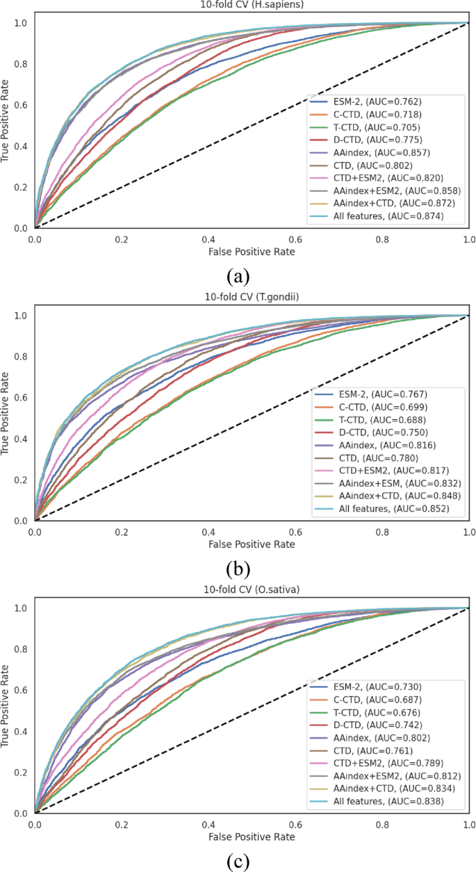

ROC curves of various feature representation methods on the 10-fold cross-validation data of (a) H. sapiens, (b) T. gondii and (c) O. sativa datasets.

Comparative evaluation of feature representation methods on test sets

To evaluate the generalization ability of the LightGBM-based Khib prediction model, 10% of each species-specific dataset was reserved as an independent test set. The model performance on these sets, using various encoding schemes and their combinations, closely aligned with the cross-validation results (Sec.”Comparative evaluation of feature representation methods on validation datasets“). Notably, AAindex encoding demonstrated stable performance across all species achieving AUC scores of 0.866 (H. sapiens), 0.828 (T. gondii), and 0.802 (O. sativa) highlighting its strong and consistent discriminative power for Khib site prediction based on physicochemical properties.

The incremental integration of complementary feature representations yielded a progressive enhancement in predictive performance across all datasets. The initial combination of CTD descriptors established a foundational improvement over individual encoding. This performance was subsequently enhanced through the sequential integration of ESM-2 and AAindex features, culminating in the comprehensive “All Features” approach that consistently demonstrated good performance across all evaluation metrics.

On the H. sapiens independent test set (Table 3), the comprehensive feature integration (“All Features”) achieved the highest performance metrics: ACC = 0.814, SN = 0.840, SP = 0.787, F1-score = 0.821, MCC = 0.629, and AUC = 0.890. Notably, the AAindex + CTD combination also demonstrated robust performance (ACC = 0.808, and AUC = 0.885), revealing that these feature types capture complementary aspects of the sequence information, particularly relevant to Khib site prediction in human proteins. The performance differential between the best individual encoding (AAindex with ACC = 0.793, and AUC = 0.866) and the optimal feature combination (“All Features”) represented a statistically significant improvement of 2.65% in accuracy and 2.77% in AUC, underscoring the value of feature integration.

For the T. gondii independent test set (Table 4), the “All Features” approach similarly demonstrated enhanced performance, achieving ACC = 0.781, SN = 0.799, SP = 0.763, F1-score = 0.781, MCC = 0.562, and AUC = 0.867. The performance enhancement from the best individual encoding (AAindex with ACC = 0.756, and AUC = 0.828) to the optimal feature combination represented an improvement of 3.31% in accuracy and 4.71% in AUC. The AAindex + ESM combination also performed well (ACC = 0.773, and AUC = 0.853), showing that the integration of physicochemical properties with evolutionary information provides valuable discriminative features for this organism.

Analysis of the O. sativa independent test set (Table 5) revealed that the “All Features” integration achieved the highest overall performance with ACC = 0.764, SN = 0.788, SP = 0.737, F1-score = 0.776, MCC = 0.526, and AUC = 0.835. Interestingly, the AAindex + CTD combination demonstrated comparable performance (ACC = 0.763, and AUC = 0.839). The performance improvement from the best individual encoding (AAindex with ACC = 0.728, and AUC = 0.802) to the optimal feature combination represented an enhancement of 4.95% in accuracy and 4.11% in AUC.

The ROC curves illustrated in Fig. 4 visually represent the performance differentials across the various feature representation methods on the independent test sets. These curves provide clear evidence for the progressive enhancement in discriminative capacity achieved through feature integration, with the “All Features” approach consistently demonstrating the largest AUC across all datasets.

The steady improvement in performance from combining features, seen in both cross-validation and independent tests, shows that different encoding methods capture useful and complementary information about protein sequences for predicting Khib sites. The integration of these complementary features provides a more comprehensive representation of the sequence characteristics, enabling more accurate and robust prediction of Khib sites across diverse organisms.

Table 3 LightGBM classification performance with different feature representation methods on the independent test set of the H. sapiens dataset. Boldface values indicate the best value for each metric.Table 4 LightGBM classification performance with different feature representation methods on the independent test set of the T. gondii dataset. Boldface values indicate the best performance for each metric.Table 5 LightGBM classification performance with different feature representation methods on the independent test set of the O. sativa dataset. Boldface values indicate the best performance for each metric.Fig. 4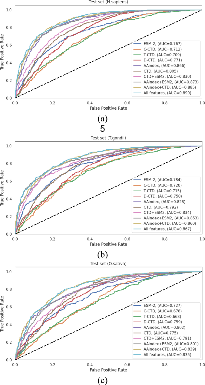

ROC curves of various feature representation methods on the independent test sets of (a) H. sapiens, (b) T. gondii and (c) O. sativa datasets.

Performance analysis of feature selection algorithms

The HyLightKhib framework has a comprehensive two-phase feature engineering strategy to optimize predictive performance. The first phase focuses on integrating diverse feature representation techniques to capture complementary aspects of protein sequences. While this integration enhances discriminative capacity, it inherently introduces potential redundancy and noise that may impair computational efficiency and model generalization. Therefore, the second phase depends on feature selection algorithms to identify the most informative feature subset, with the primary objective of reducing computational overhead, while preserving model accuracy.

To identify the most effective dimensionality reduction approach, we systematically evaluated five established feature selection techniques: ANOVA, RFE, Lasso, Elastic Net, and MI. The evaluation was conducted across three species-specific datasets (H. sapiens, T. gondii, and O. sativa), with performance assessed through rigorous 10-fold cross-validation detailed in supplementary material Table S10, and independent test set validation Table S11.

The original integrated feature set comprised 1,487 dimensions. Systematic evaluation across H. sapiens feature subsets from 100 to 1,000 features revealed that performance plateaus beyond 600 features, with cross-validation AUC values remaining stable (0.872–0.873) across the 600–1000 feature range (Fig. 5). While the maximum AUC (0.873) was achieved at 900 features, the performance difference from that obtained with 700 features was minimal (0.001 AUC units) and not statistically significant (p = 0.31). We selected 700 features as the optimal balance between performance and computational efficiency, as this threshold achieved 99.8% of the maximum performance level, while representing 83.2% of total mutual information variance. This leads to a reduction of the computational overhead by 22% compared to the case of 900 features.

Fig. 5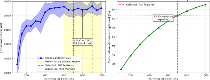

Systematic optimization for mutual-information-based feature selection threshold.

As detailed in Table 6, MI-based feature selection achieved balanced dimensionality reduction across all three feature categories (ESM, CTD, and AAindex), but with species-specific variations in the proportional representation of each category. For the H. sapiens dataset, the original 1,487 dimensions were reduced to 700, with proportional contributions of ESM (34.14%), CTD (9.29%), and AAindex (56.57%). The T. gondii dataset exhibited a slightly different distribution, with ESM features constituting a larger proportion (40.14%) compared to H. sapiens. CTD features maintained a similar contribution (8.57%), and AAindex features represented a somewhat smaller proportion (51.29%). For the O. sativa dataset, the distribution more closely resembled that of H. sapiens, with ESM, CTD, and AAindex features contributing 33.86%, 10.29%, and 55.86%, respectively.

These differential distributions, visualized in Fig. 6, provide valuable insights into the relative importance of different feature categories across species. The fact that a large share of AAindex features (51.29–56.57%) was chosen in all datasets highlights how important physicochemical properties are for predicting Khib sites. This matches the strong results AAindex gave when used alone, as shown in Sec.”Comparative evaluation of feature representation methods on validation datasets” and “Comparative evaluation of feature representation methods on test sets“. The varying contribution of ESM features, particularly the higher proportion in T. gondii (40.14%) compared to those of H. sapiens (34.14%) and O. sativa (33.86%), reveals potential species-specific variations in the relevance of evolutionary information for Khib site prediction.

Elastic Net achieved more substantial dimensionality reductions through its inherent regularization mechanism, decreasing the feature dimensionality to 532, 446, and 447 for H. sapiens, T. gondii, and O. sativa, respectively. This more aggressive feature reduction did not consistently translate to advanced performance, highlighting the critical balance between dimensionality reduction and information preservation.

Table 6 Summary of the feature representation methods and their dimensionality before and after MI feature selection.Fig. 6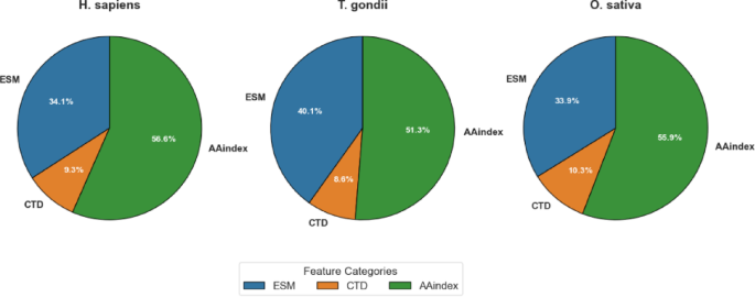

Visualization of feature category contribution after MI selection by dataset.

The performance metrics of the various feature selection methods on the independent test sets are comprehensively presented in Table S11. These results reveal several significant patterns and insights regarding the efficacy of feature selection in enhancing model performance.

For the H. sapiens dataset, the original feature set established a robust baseline with an ACC of 0.814 and an AUC of 0.890. Among the feature selection methods, MI demonstrated effective performance, achieving comparable results with an ACC of 0.816 and an AUC of 0.893 while utilizing only 47% of the original features. ANOVA similarly achieved an AUC of 0.893, albeit with a slightly lower ACC of 0.801. The other methods maintained comparable performance levels, with Elastic Net showing modest improvement (ACC of 0.804 and AUC of 0.888) while achieving the most substantial dimensionality reduction. These results demonstrate that for the H. sapiens dataset, feature selection successfully maintains predictive performance while substantially reducing computational complexity.

Analysis of the T. gondii dataset revealed that the original feature set achieved an ACC of 0.781 and an AUC of 0.867. Both RFE and MI demonstrated enhanced discriminative capacity, with AUC values of 0.874 and 0.876, respectively.  The MI achieved notable performance metrics (ACC of 0.782, MCC of 0.551 and AUC of 0.876) over the original feature set while reducing dimensionality. Lasso demonstrated the most conservative performance among the methods evaluated (ACC of 0.759, and AUC of 0.851), revealing that its aggressive sparsity-inducing mechanism may eliminate some informative features for this particular organism. Elastic Net, with its balanced regularization approach, achieved performance metrics (ACC of 0.782, AUC of 0.866) comparable to those of the original feature set while requiring substantially fewer features.

For the O. sativa dataset, MI consistently achieved the highest performance among all evaluated methods, with an ACC of 0.765, an MCC of 0.517, and an AUC of 0.847. This performance represented an improvement over the original feature set (ACC of 0.764 and AUC of 0.835). The remaining feature selection methods demonstrated varying degrees of effectiveness, with ANOVA, RFE, and Elastic Net providing modest enhancements in specific metrics while maintaining an overall performance comparable to that of the original feature set. Lasso demonstrated the most substantial performance differential among the evaluated methods, achieving an ACC of 0.757 and an AUC of 0.829, ensuring potential species-specific variations in the effectiveness of sparsity-inducing feature selection.

The ROC curves illustrated in Fig. 7 represent the performance differentials across the various feature selection methods for all three species datasets. These curves corroborate the quantitative metrics presented in Table S11, demonstrating the consistently notable performance of MI-based feature selection across all datasets. The comprehensive evaluation reveals that while the original feature set provides robust baseline performance, feature selection methods successfully maintain or enhance predictive performance while substantially reducing computational complexity. MI-based feature selection achieved the highest performance metrics across all three datasets while reducing feature dimensionality by approximately 47%, effectively capturing nonlinear relationships between features and class labels.

Fig. 7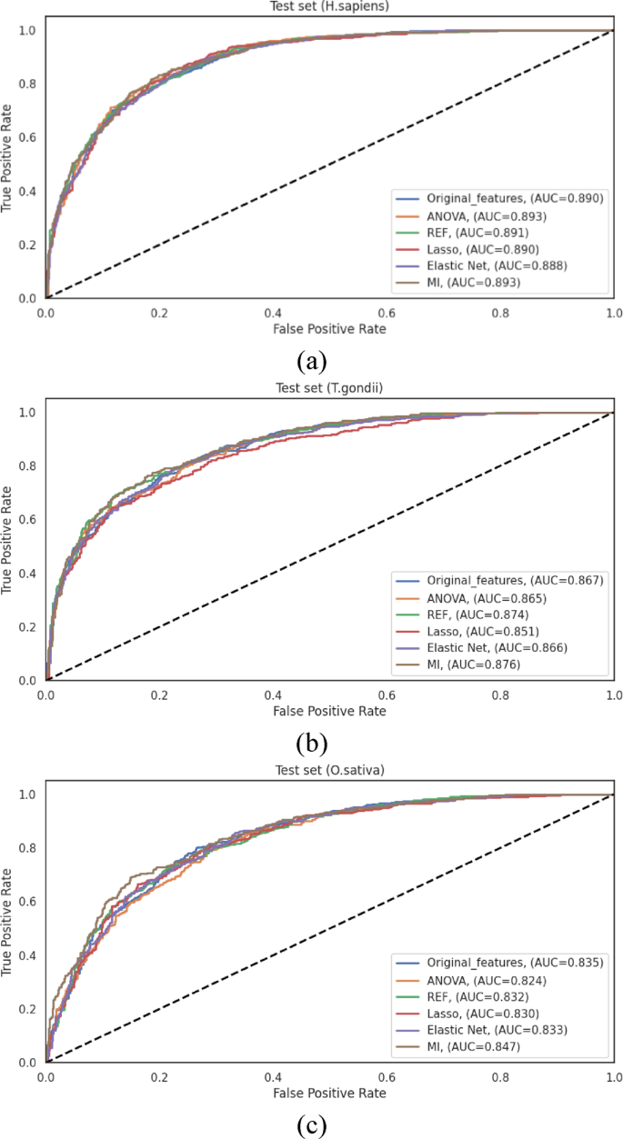

ROC curves illustrating the performance of LightGBM using different feature selection algorithms on the independent test sets of (a) H. sapiens, (b) T. gondii, and (c) O. sativa datasets.

Performance evaluation of machine learning classifiers

Having established the optimal feature representation approach and identified MI-based feature selection as the most effective dimensionality reduction technique, we evaluated the performance of various machine learning algorithms for Khib site prediction. This comparative analysis encompassed seven widely-used classification algorithms: K-Nearest Neighbours (KNN) 70, Adaptive Boosting (AdaBoost) 71, Random Forest (RF) 72, Support Vector Machine (SVM) 73, XGBoost, CatBoost, and LightGBM. The evaluation was systematically conducted across the three species-specific datasets (H. sapiens, T. gondii, and O. sativa), utilizing the MI-selected feature subsets as input for each classifier.

To ensure a rigorous and fair comparison, each classifier hyperparameters were optimized through grid search cross-validation 74. The final configurations were as follows: KNN was employed with the Euclidean distance metric with k = 9 neighbors; RF was based on the Gini impurity criterion for node splitting with an ensemble of 500 decision trees; AdaBoost was implemented with a learning rate of 1.0 and 500 weak learners; SVM was employed with a polynomial kernel function; XGBoost was configured with a learning rate of 0.1, maximum tree depth of 15, 500 estimators, and both L1 and L2 regularization (λ = 1 and λ = 2, respectively); CatBoost was implemented with default hyperparameters and 500 iterations; and LightGBM was configured as detailed in Table 2. This systematic optimization strategy ensures that each algorithm performance was evaluated under optimal operating conditions.

To ensure robust performance assessment, we implemented a dual validation strategy employing 10-fold cross-validation and independent test set evaluation. The cross-validation results are documented in Table S12. These results complement the independent test set evaluation presented in Table S13 and visualized in Fig. 8, offering a more comprehensive assessment of classifier performance across diverse data scenarios.

For the H. sapiens dataset, LightGBM achieved the highest performance among all evaluated classifiers, with an ACC = 0.816 and an AUC = 0.893. CatBoost followed closely with ACC = 0.807 and AUC = 0.886, and XGBoost performed competitively with ACC = 0.793 and AUC = 0.878. The traditional algorithms, SVM, RF, and AdaBoost, exhibited moderate performance, with AUC values of 0.848, 0.843, and 0.840, respectively. KNN demonstrated substantially lower discriminative capacity (AUC = 0.776), showing that distance-based classification approaches may be less suitable for this prediction task. The performance differential between LightGBM and KNN (AUC difference of 0.117) underscores the significant impact of algorithm selection on predictive efficacy for human Khib sites.

Analysis of the T. gondii dataset revealed similar performance patterns, with LightGBM achieving the highest overall metrics (ACC = 0.782 and AUC = 0.876). CatBoost (AUC = 0.868) and XGBoost (AUC = 0.864) demonstrated comparable performance, indicating that gradient-boosting algorithms generally excel at capturing the complex patterns associated with Khib sites in this organism. SVM maintained competitive performance with AUC = 0.841, while RF and AdaBoost exhibited moderate discriminative capacity with AUC = 0.831, and 0.836, respectively. As observed in the H. sapiens dataset, KNN achieved notably lower performance with AUC = 0.751, providing further evidence of the limitations of distance-based approaches for this prediction task.

The O. sativa dataset analysis reinforced the patterns observed in the other organisms, with LightGBM consistently achieving the highest performance among all classifiers with ACC = 0.765 and AUC = 0.847. CatBoost (AUC = 0.833) and XGBoost (AUC = 0.821) maintained their competitive performance, followed by SVM (AUC = 0.804). The ensemble-based approaches, RF and AdaBoost, demonstrated moderately lower performance with AUC = 0.787 and 0.784, respectively, while KNN exhibited the lowest discriminative capacity with AUC = 0.693. The substantial performance differential between LightGBM and KNN was most pronounced in this dataset, showing that the selection of an appropriate classification algorithm is particularly critical for plant Khib site prediction.

The consistent performance of LightGBM across all species datasets, validated by both cross-validation and independent testing, stems from its architectural strengths tailored to complex feature spaces like those in Khib site prediction. Its histogram-based binning enhances efficiency in handling high-dimensional data, while the leaf-wise tree growth with depth control captures complex nonlinear patterns without overfitting. Additionally, robust regularization contributes to its strong generalization ability. Although CatBoost and XGBoost also performed well, LightGBM consistently outperformed them, indicating that its specific design choices offer a distinct advantage for this classification task.

Fig. 8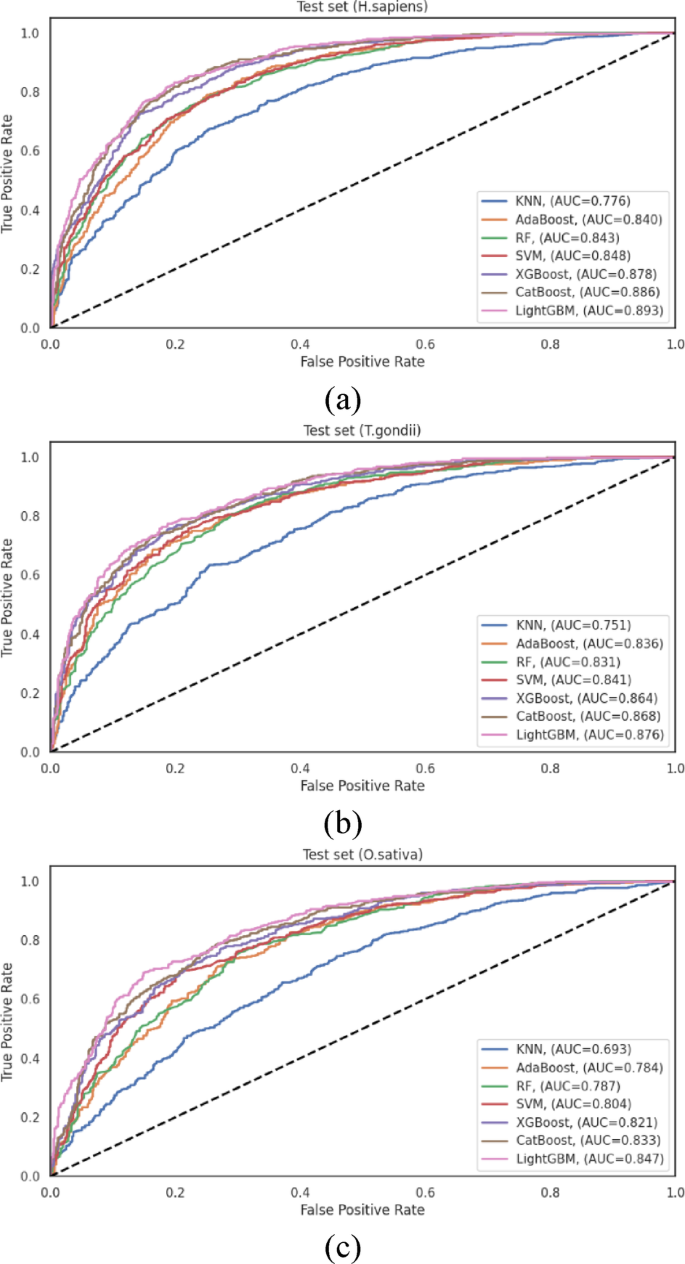

ROC curves showing the performance of different machine learning classifiers on the independent test sets of (a) H. sapiens, (b) T. gondii and (c) O. sativa datasets.

Visualization of feature learning and cluster separation analysis

To evaluate HyLightKhib discriminative capacity, t-distributed stochastic neighbor embedding (t-SNE)75 was employed to visualize the feature transformation capabilities of the framework. The visualization analysis utilized the optimal configuration identified through a comprehensive performance evaluation, incorporating original input features with LightGBM classification following MI-based feature selection to maintain consistency with the best-performing model architecture.

The t-SNE visualizations for the species-specific H. sapiens, T. gondii, and O. sativa datasets shown in Fig. 9 demonstrate the effectiveness of our optimized framework in transforming the hybrid features into highly discriminative probability predictions. To provide a quantitative assessment beyond visual interpretation, silhouette scores and Davies-Bouldin indices were calculated for both the original feature space (left panels) and the LightGBM probability predictions (right panels).

The silhouette score measures how similar data points are to their cluster compared to other clusters, with values ranging from − 1 to 1, where higher values indicate better-defined clusters. Scores near 0 indicate overlapping clusters, while negative values indicate potential misclassification. The Davies-Bouldin index quantifies the average similarity between clusters, where lower values indicate better separation with more compact and well-separated clusters. Values closer to 0 represent optimal clustering quality.

For the H. sapiens dataset (Fig. 9a), the original feature space exhibited minimal class separation with a silhouette score of 0.008 and Davies-Bouldin index of 1.200, indicating substantial overlap between Khib-modified and non-modified lysine residues even after feature selection. The LightGBM probability predictions achieved substantial improvement with a silhouette score of 0.262 and the Davies-Bouldin index of 0.885. This improvement in silhouette score demonstrates the LightGBM ability to transform the original features into highly discriminative predictions.

The T. gondii dataset analysis (Fig. 9b) revealed the most pronounced discriminative transformation, with LightGBM probability predictions achieving a silhouette score of 0.285 and Davies-Bouldin index of 0.686 compared to those of the input features (silhouette score of 0.005, and Davies-Bouldin index of 1.100). This improvement in cluster separation metrics aligns with the 87.6% AUC performance reported in Sect. 3.5, demonstrating the LightGBM capacity to extract discriminative patterns from the optimally-selected feature subset for this organism.

For the O. sativa dataset (Fig. 9c), the LightGBM transformed the input features into probability predictions with a silhouette score of 0.205 and Davies-Bouldin index of 0.831, representing an improvement over the input feature space (silhouette score of 0.006, and Davies-Bouldin index of 1.163). This improvement confirms the LightGBM effectiveness in processing the input feature set for plant protein analysis.

Fig. 9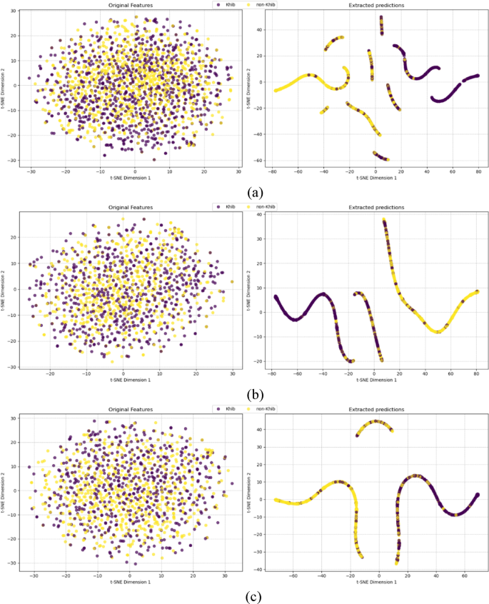

t-SNE visualization of input features (left) and extracted predictions (right) by HyLightKhib of (a) H. sapiens, (b) T. gondii and (c) O. sativa datasets.

Comparative motif analysis and position-specific amino acid preferences

To further investigate the sequence characteristics underlying Khib site recognition and the varying classification performance across organisms, Two-Sample Logo analysis 76 was employed to identify position-specific amino acid preferences surrounding modification sites. The Two-Sample Logo is a statistical visualization tool that compares amino acid composition between two sequence sets (positive and negative samples) by calculating the difference in relative frequencies at each position and assessing statistical significance through hypothesis testing.

The Two-Sample Logo analysis was performed using a 43-residue window (−21 to + 21 positions relative to the central lysine) for all three species datasets. At each position, amino acid frequencies were compared between Khib-modified and non-modified sequences using a two-sample t-test with a significance threshold of p-value ≤ 0.05. The resulting logos display amino acids with statistically significant differences in their occurrence frequencies between the two sample groups.

Enriched amino acids represent residues that occur more frequently in Khib-modified sequences compared to non-modified sequences at specific positions, showing positive associations with modification propensity. Conversely, depleted amino acids represent residues that occur less frequently in Khib-modified sequences, indicating negative associations with modification likelihood. The height of each letter is proportional to the magnitude of the frequency difference, with larger letters indicating more statistically significant and biologically relevant associations.

Two-sample logo analysis across three taxonomically diverse species reveals an evolutionary conservation of Khib recognition mechanisms alongside organism-specific adaptations. For H. sapiens (Fig. 10a), lysine (K) enrichment in upstream positions (−21 to −1) and glutamic acid (E) enrichment recommend cooperative recognition mechanisms within lysine-rich regions and favourable electrostatic environments for enzymatic machinery. Consistent proline (P) depletion indicates preferential modification in structured regions rather than helix-disrupted areas.

The T. gondii dataset (Fig. 10b) demonstrates conserved K enrichment patterns while exhibiting parasite-specific adaptations, including distinctive alanine (A) enrichment and reduced glutamic acid prominence compared to human sequences. Extensive serine (S) depletion (−8 to −10%) recommends spatial segregation mechanisms preventing phosphorylation-Khib crosstalk, while maintained proline depletion reinforces structured region preference.

Plant-specific adaptations in O. sativa (Fig. 10c) maintain core recognition features with pronounced E enrichment exceeding T. gondii levels, indicating enhanced acidic residue requirements in plant Khib systems. Unique arginine (R) depletion patterns (−6 to −8%) alongside consistent proline reduction recommend the avoidance of excessive positive charge density and structural disruptions.

Quantitative analysis reveals hierarchical motif signatures correlating directly with computational performance. Maximum lysine enrichment decreases across H. sapiens (14.5%), T. gondii (13.5%), and O. sativa (12.7%), corresponding precisely to classification performance with 89.3%, 87.6%, and 84.7% AUC, respectively.

Fig. 10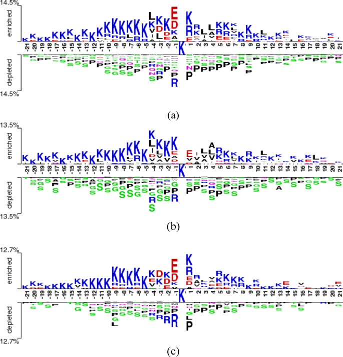

Comparison of the amino acid preferences near the Khib sites in the (a) H. sapiens, (b) T. gondii and (c) O. sativa datasets.

Comparative analysis with state-of-the-art Khib prediction methods

To evaluate the performance of the HyLightKhib model in identifying Khib sites, its results were compared with those of existing Khib prediction tools: iLys-Khib, KhibPred, DeepKhib and ResNetKhib. iLys-Khib used a 35-residue window centred on the lysine and a fuzzy SVM. This approach reduces noise by giving different weights (fuzzy memberships) to samples depending on how relevant they are and how close they are to the class center. It incorporates three feature encoding methods: Amino Acid Factors (AAF), Binary Encoding (BE), and the Composition of k-spaced Amino Acid Pairs (CKSAAP) to capture the sequence context surrounding Khib sites. Feature selection used the maximum Relevance Minimum Redundancy (mRMR) method to retain the most informative features.

KhibPred used the same feature encoding as iLys-Khib but with a smaller window size of 29. It also used an ensemble SVM classifier to handle the imbalance in the dataset, where Khib sites are fewer than non-Khib sites. To handle this issue, the negative samples were divided into seven subsets, with an individual SVM trained on each subset, then combined with the positive samples. The ensemble model aggregated the predictions from all SVMs to make the final classification.

DeepKhib is a deep learning framework that employs a CNN architecture with a one-hot encoding approach. The model utilizes a four-layer architecture consisting of an input layer with one-hot encoding representation, a convolution layer containing four convolution sublayers (with 128 filters each of lengths 1, 3, 9, and 10) and two max pooling sublayers, a fully-connected layer incorporating global average pooling to prevent overfitting, and an output layer with sigmoid activation function for probability scoring.

ResNetKhib is the first cell-type-specific deep learning predictor for lysine Khib sites, employing a residual neural network (ResNet) architecture with a one-dimensional convolution and transfer learning strategy across different cell types and species. The model architecture consists of five key components: an input layer, an embedding layer, a convolution module containing six blocks with residual connections (first block with 64 filters, followed by five residual blocks), a fully-connected layer with 16 neurons for feature flattening, and an output layer with sigmoid activation for probability scoring. Both DeepKhib and ResNetKhib have 37-residue windows.

For a comprehensive methodological comparison, the SVM models documented in the iLys-Khib and KhibPred publications 25,26 and the CNN architectures described in DeepKhib and ResNetKhib 6,28 were reimplemented according to their original specifications. These models were subsequently trained and evaluated using our curated datasets under identical experimental conditions as our proposed method, thereby ensuring a fair and direct comparison. This approach eliminates potential confounding variables that might arise from differences in data preprocessing, partitioning strategies, or evaluation metrics.

Model training was performed using consistent cross-validation protocols across all compared methods, and performance was assessed on the same independent test sets to provide an unbiased evaluation of predictive capabilities. The comparative evaluation results across all benchmark methods are presented in Table S14.

As shown in Table S14, HyLightKhib achieved accuracy improvements of approximately 16.1%, 15.5%, 6.1%, and 2.9% over iLys-Khib, KhibPred, DeepKhib, and ResNetKhib, respectively, for the H. sapiens dataset. The improvements for the T. gondii dataset were 9.5%, 8.9%, 1.3%, and 0.6% compared to the same methods. For the O. sativa dataset, HyLightKhib achieved accuracy improvements of 13.8%, 11.35%, 8.7%, and 4.8% compared to the aforementioned predictors.

The ROC curves and the corresponding AUC values presented in Fig. 11 reveal more modest improvements, particularly compared to recent deep learning methods. HyLightKhib achieved AUC values of 0.893, 0.876, and 0.847 for H. sapiens, T. gondii, and O. sativa, respectively. When compared to ResNetKhib, the most competitive baseline method, the AUC improvements were 1.8%, 2.4%, and 3.0% for the three datasets, respectively.

Fig. 11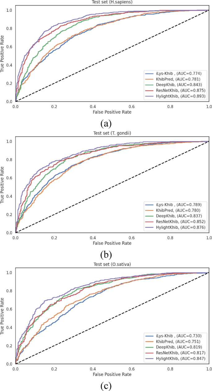

ROC curves comparing existing Khib predictors and HyLightKhib on the independent test sets for (a) H. sapiens, (b) T. gondii, and (c) O. sativa datasets.

The statistical significance of AUC differences was assessed using the Hanley & McNeil method 77 for comparing correlated ROC curves derived from identical test sets. Although newer methods such as DeLong’s 78 test are now common, Hanley & McNeil remains a valid approach for estimating the significance of AUC differences in diagnostic and predictive modeling. Using this method, HyLightKhib demonstrated highly-significant improvements (p 

For the H. sapiens dataset, significant improvements were observed over ResNetKhib (p = 7.47 × 10⁻¹¹), DeepKhib (p p p T. gondii dataset showed highly significant improvements over ResNetKhib (p = 6.11 × 10⁻¹⁰), DeepKhib (p p p O. sativa dataset exhibited the same pattern with significant improvements over ResNetKhib (p = 8.23 × 10⁻¹²), DeepKhib (p p p 

However, the primary advantage of HyLightKhib lies in its computational efficiency rather than dramatic performance gains. A comprehensive computational efficiency analysis was conducted to quantitatively assess the practical applicability of HyLightKhib compared to existing models. All experiments were performed on a standard desktop system (AMD Ryzen 5 7520U, 2.80 GHz, and 16.0 GB RAM). As detailed in Table 7, HyLightKhib demonstrates computational advantages across all evaluated metrics.

HyLightKhib demonstrated enhanced computational efficiency across all three datasets, with training times of 19.95, 19.36, and 21.77 seconds for the H. sapiens, T. gondii, and O. sativa datasets, respectively. When compared to existing methods, HyLightKhib achieved substantial training speedups: 92-166 times faster than DeepKhib (1994.11–3321.92 seconds), 19-27 times faster than ResNetKhib (414.59–548.05 seconds), 347-528 times faster than KhibPred (7236.3–10541.27 seconds), and 16–40 times faster than iLys-Khib (311.69–793.69 seconds). The most pronounced efficiency gains were observed against the ensemble-based KhibPred, highlighting HyLightKhib’s streamlined architecture.

Memory utilization analysis revealed HyLightKhib resource-efficient design, with peak consumption ranging from only 1.61–6.10 megabytes (MB) across all datasets. This represents substantial memory reductions compared to all baseline methods: 33-127 times less than DeepKhib (73.79-378.34 MB), 49-75 times less than ResNetKhib (121.07-298.23 MB), 42-109 times less than KhibPred (174.9-254.77 MB), and 10-121 times less than iLys-Khib (50.21–194.00 MB). The minimal memory footprint makes HyLightKhib particularly suitable for deployment in resource-constrained environments.

Inference performance evaluation demonstrated HyLightKhib capability for high-throughput applications, processing individual samples in 0.021–0.046 seconds across all datasets. This translates to significant inference accelerations: 63-132 times faster than DeepKhib (2.51–3.84 seconds), 24-48 times faster than ResNetKhib (1.014–1.29 seconds), 131-433 times faster than iLys-Khib (5.31–12.57 seconds), and remarkably 2139-4677 times faster than KhibPred (98.21–99.74 seconds). These performance metrics underscore HyLightKhib practical advantage for large-scale proteome-wide Khib site prediction tasks.

These quantitative computational benchmarks provide compelling empirical evidence for practical advantages in real-world applications. The significant reduction in computational resources, while maintaining competitive accuracy, makes HyLightKhib particularly suitable for large-scale proteomic analyses and integration into high-throughput experimental workflows. This empirical evaluation demonstrates that HyLightKhib offers an optimal balance between predictive performance and computational efficiency.

Table 7 Comparative analysis of computational efficiency metrics for Khib site prediction models across different dataset sizes.