Data
We draw weekly mortality data from the Eurostat database (data code ‘demo_r_mweek3’). Different regions make data available over different time periods; we limit our analysis to 2015–2019 to match the most common period of data availability, following other work35. Where possible, we use all-age, all-sex mortality rates from NUTS3 (third administrative level below country) regions, except in Germany, where we only have these data at the NUTS1 level. This yields a total of 924 regions with continuous mortality rate data over 2015–2019. Age-group-specific rates (for example, over 65 years) are available for only a slightly smaller number of regions (n = 908), so we use all-age rates to maximize coverage in our preferred specification.
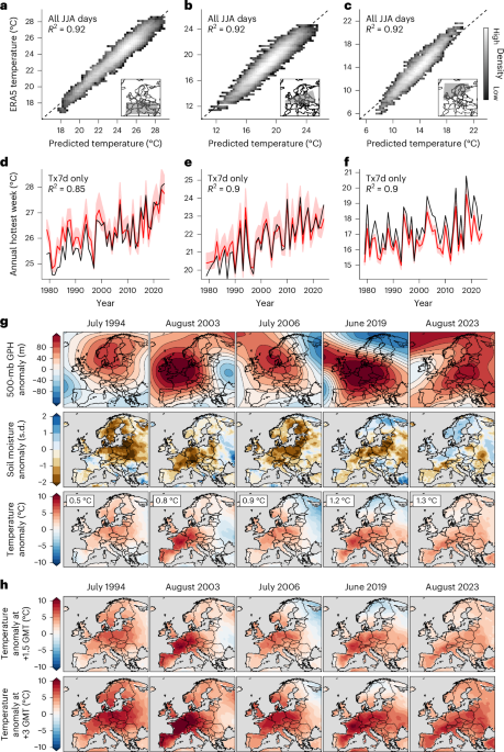
Our historical climate data come from the E-OBS station-based dataset50 and the ERA5 reanalysis51. We use E-OBS daily surface temperature when possible, including for the initial definitions of each extreme event and the mortality calculations. E-OBS data are spatially averaged to the appropriate NUTS regions, weighting grid cells within regions by the population of each grid cell. We use ERA5 for the out-of-sample machine learning predictions (Fig. 1) and maps of historical meteorological conditions (Fig. 1).
Counterfactual extreme heat events
We use a machine learning architecture recently developed and validated by ref. 38 to produce counterfactual versions of historical extreme heat events. Following this approach, we train CNNs on an ensemble of GCM realizations, with the goal of predicting daily mean temperature anomalies over a specified region given daily meteorological conditions and the annual GMT anomaly.
The predictors for each day are daily sea level pressure (SLP), daily GPH fields at the 700-mb, 500-mb and 250-mb levels, daily soil moisture between 0 cm and 10 cm, the calendar day, an indicator variable for each GCM and the GMT anomaly over the previous 12 months. Before training, the meteorological predictors are detrended with respect to the grid cell, calendar day and GMT and then standardized by subtracting the grid-cell calendar-day mean and dividing by the grid-cell calendar-day standard deviation38. The detrended and standardized surface pressure, GPH and soil moisture are the factors we refer to as ‘meteorological conditions’ throughout the text. Using detrended and standardized anomalies in this process means that these meteorological conditions explain day-to-day variation in temperature, but do not contain the signal of global warming. Daily mean temperature anomalies (the predictands) are referenced to the 1979–2023 period, with GMT anomalies relative to the same period when used in training. However, we note that throughout the text we refer to GMT anomalies relative to 1850–1900.
In our experimental setup, we train the CNN on a pooled set of CMIP6 simulations: three realizations each of five GCMs (CanESM5, HadGEM3-GC31-LL, MIROC6, MPI-ESM1-2-LR and UKESM1-0-LL). We combine the historical and shared socioeconomic pathway (SSP) 5-8.5 simulations to create a 1850–2100 dataset for each realization. These five GCMs are chosen because they each archive three-dimensional daily atmospheric fields of each input variable from several realizations of the GCM. While these data requirements prevent us from using a wider range of CMIP6 models, these five GCMs are representative of the range of climate sensitivities in the CMIP6 ensemble52. Since this analysis focuses on summer heat waves, we train each CNN on CMIP6 data from May through September.
We then apply the model to predict daily temperature anomalies using predictor data from ERA5. One set of predictions uses the observed GMT time series, whereas the other sets use counterfactual GMT values but maintain the other daily predictors from the reanalysis. The result is a set of counterfactual temperature time series that maintain realistic day-to-day weather conditions but vary according to the annual GMT anomaly. While we train the CNN on a pooled set of realizations, we include an indicator variable for each GCM which allows the CNN to make separate predictions based on differences between individual GCMs. This indicator variable is one-hot encoded and provided to the neural network after the convolutional layers along with the calendar day and GMT inputs (similar to ref. 38). In training, we also vary the random seed five times to account for random differences in model training. This procedure yields 25 total predictions for each counterfactual event and GMT anomaly, five random seeds each for five GCMs.
We use a ‘delta’ method to apply the CNN predictions to E-OBS gridded observations. For each day in the event of interest, we take the difference between the counterfactual CNN predictions on that day and the original CNN predictions for that day using the actual GMT. We then apply these deltas to the E-OBS observed data for that day to calculate counterfactual daily time series. Finally, we aggregate these counterfactual gridded daily temperature data into averages at the NUTS region level as with the original observations.
In ref. 38, the CNNs were trained to predict temperature in regions chosen for their relevance to specific historical extremes. In our application, we would like to apply these predictions to a set of events, each with slightly different spatial footprints. We therefore train the CNNs to predict temperature change on land in each of three regions as defined by the IPCC: the Mediterranean, Western and Central Europe and Northern Europe53. The events manifest differently in each of these regions, with temperatures generally highest in the Mediterranean region and lowest in Northern Europe (Supplementary Fig. 4). We then apply the deltas for each region uniformly to the grid cells within each region. When training the CNNs, the input SLP, GPH and soil moisture fields are defined by broader regions of approximately 35° latitude and 85° longitude centred on the IPCC regions38.
Exposure–response functions
We use panel regression with fixed effects to measure the causal effect of temperature on mortality across Europe. This widely used approach11,12,54,55,56 involves regressing mortality rates on a nonlinear function of temperature, along with vectors of intercepts (fixed effects) that non-parametrically remove seasonal or annual average factors separately for each region.
We also account for heterogeneity across regions by interacting temperature with the 2000–2019 average temperature of each region, allowing the temperature exposure–response curve to vary on the basis of the long-term climate of a region. This approach leverages cross-sectional variation in temperature to assess societal adaptation to extreme heat, in effect asking whether the same temperature level has a different effect in a region that is warmer on average than a region that is cooler on average. Cross-sectional variation is less amenable to causal identification since there may be other factors (for example, income and demographics) that are correlated with both average temperature and heat sensitivity. Nevertheless, assessing heterogeneity by mean temperature is a well-established strategy for identifying present and future climate adaptation11,57,58,59,60, so we adopt it here while acknowledging the potential for additional relevant axes of heterogeneity. Our approach is also similar to multistage methods that have been used in other recent papers to estimate variation in exposure–response functions (for example, refs. 13,61,62), although we run a single regression that accommodates variations across regions rather than pooling time-series regressions from separate regions.
Specifically, we estimate the following regression relating contemporaneous and lagged temperature T to log mortality rates M in region i, week w and year y with ordinary least squares:
$${M}_{iwy}=\mathop{\sum }\limits_{j=0}^{L}[\,f({T}_{i(w-j)y})+f({T}_{i(w-j)y})\times {\bar{T}}_{i}]+{\mu }_{iy}+{\delta }_{iw}+{\epsilon }_{iwy}$$
(1)
The region–year fixed effects \({\mu }_{{iy}}\) and region–week fixed effects \({\delta }_{{iw}}\) remove the influence of long-term trends and seasonal cycles that could confound the temperature–mortality relationship and do so separately for each region. The \({\bar{T}}_{i}\) term denotes the 2000–2019 mean temperature in each region i. We estimate distributed lag models that sum the impact on mortality of contemporaneous and lagged temperature exposure, with j indexing weekly lags. As discussed below, our main model uses 3 weeks of lagged temperatures. Regressions are weighted by the population of each region.
A key consideration is that mortality rates are provided at the weekly scale but temperature extremes can impact mortality rates on daily timescales. We require a strategy that preserves daily nonlinearities while matching the weekly scale of the mortality data. We thus follow previous work11 and sum the daily mean temperature from each day d within week w after a fourth-order polynomial transformation has been applied to the temperature of each day:
$$f({T}_{iwy})={\beta }_{1}\mathop{\sum }\limits_{d=1}^{7}{T}_{iw(d)y}+{\beta }_{2}\mathop{\sum }\limits_{d=1}^{7}{T}_{iw(d)y}^{2}+{\beta }_{3}\mathop{\sum }\limits_{d=1}^{7}{T}_{iw(d)y}^{3}+{\beta }_{4}\mathop{\sum }\limits_{d=1}^{7}{T}_{iw(d)y}^{4}$$
(2)
We estimate independent coefficients for each of the summed polynomial terms in equation (2). Because weekly mortality rates are the sum of daily mortality rates (given constant population), calculating the effects of daily sums preserves the nonlinear effect of each individual day on weekly mortality rates. We use daily mean temperature following earlier work11, but using daily maximum or daily minimum temperatures yields only small differences in exposure–response functions (Supplementary Fig. 7).
We use lags in the regression to incorporate delayed effects of temperature. These delayed effects could arise simply as a result of additional mortality if people die several days after heat exposure. They could also manifest as ‘displacement’ or ‘harvesting,’ where mortality is abnormally low after heat waves since the heat accelerated the deaths of people who would have died soon regardless of the heat. Indeed, we do observe some displacement following the events (Fig. 3), as the lag-2 and lag-3 regression coefficients are negative (Supplementary Fig. 9). We use three lags in our main analysis following earlier work35, but re-estimating the model using six lags yields similar results, with potentially slightly more displacement in additional weeks (Supplementary Fig. 9).
Our main regression is estimated over 2015–2019, as the period over which the greatest number of regions have continuous mortality data. Alternatively, we estimate the regression using all observations from 2000–2019, although different regions have different numbers of observations over this period. We find a very similar response, although the mortality response to high temperatures is slightly stronger when including data further back in time (Supplementary Fig. 7), consistent with other evidence of moderate adaptation to heat over this period31,49. Because the 2015–2019 sample uses a balanced set of regions with continuous data and accounts for previous adaptation to heat, we use it in our main analysis.
When we test an additional interaction with income (Supplementary Fig. 8), we calculate income as the 2000–2019 mean of log annual gross domestic product (GDP) per capita. GDP per capita is defined in Euros, GDP-deflated to account for inflation and purchasing-power-parity adjusted.
Calculating counterfactual mortality
Our central calculation compares a series of abnormally hot days at a given GMT level to a long-term mean baseline without global warming (Extended Data Fig. 2). We perform this calculation by applying the exposure–response function (Fig. 2) to the temperature time series in each region and comparing it to the same prediction when applied to the baseline time series. Because our outcome is log mortality, the difference between each prediction yields a percentage change in mortality due to experiencing the temperature at each GMT instead of the baseline temperature. We then multiply this percentage change by the average number of deaths in each region observed over 2015–2019 to calculate the additional mortality from each event. Because these deaths are relative to an underlying baseline number of deaths, we refer to them as ‘excess deaths’ or ‘excess mortality.’
Note that we generally refer to the events predicted by the machine learning method for different GMT anomalies as ‘counterfactual’ events, whereas we use ‘baseline’ to refer to a long-term average without the event.
One key methodological question in this procedure is the construction of the baseline temperature from which excess deaths are calculated. We are interested in the total number of excess deaths associated with each event, not just those caused by climate change. We therefore construct a baseline which does not include either climate change or extreme heat events. This is done in two steps:
-
(1)
We use the machine learning approach described above to construct counterfactual estimates for every summer day between 1980 and 2023 at 0 °C GMT. We subtract the ‘delta’ from this procedure from the E-OBS observations to construct a counterfactual dataset at 0 °C over the entire observational time period (that is, not just for each event). This yields a 44-year counterfactual temperature time series for each region that includes daily weather variability and extreme heat events, but not the influence of climate change.
-
(2)
We then take the long-term average across 1980–2023 from this counterfactual time series for each calendar day in each region.
The result of this calculation is an estimate of the average seasonal cycle in each region at an annual GMT anomaly of 0 °C. Because the influence of climate change was removed from these observed temperatures, this baseline does not include global warming, and because it was averaged over all years for each calendar day, it does not include deviations from the seasonal cycle (that is, it does not include extreme heat events). The black dashed line in Extended Data Fig. 2 shows the Europe-wide average of these baseline temperatures over the time period of each event.
Adaptation to climate change
Our regression approach (equation (1)) accounts for current adaptation to heat by allowing exposure–response functions to vary according to the 2000–2019 mean temperature of the region. This approach assumes that vulnerability to temperature during the 2015–2019 data period fully reflects efficient levels of adaptation investment (such as installing air conditioning, taking indoor jobs rather than working outdoors or implementing heat action plans in cities), justifiable on the basis of longer-term (2000–2019) exposures. In the future, especially in light of rising incomes, we might expect additional such actions, which could reduce the death toll that we project.
We project future adaptation under the assumption that changes in the long-run mean temperatures of regions directly translate into additional adaptation actions. We thus require an estimate of future long-run (20-year) mean temperature in each region, with which to adjust the exposure–response functions (Fig. 2). However, our approach predicts event intensity using annual global temperature, a quantity which does not directly translate into local mean temperatures over the previous 20 years. Therefore, we adopt a pattern scaling approach, following the IPCC Sixth Assessment report63, to simulate increased 20-year mean temperatures in each European subnational district depending on a given annual GMT. We use 27 models from the CMIP6 (ref. 64), spanning the historical and SSP3-7.0 experiments65. For each year, we calculate GMT anomalies (relative to 1850–1900) and local mean temperature anomalies over the previous 20 years for each European region (relative to 2000–2019). For example, for 2069 in the region that encompasses Berlin, we have the GMT change in 2069 and the regional mean temperature change over 2049–2068. The relationship between these two quantities yields a coherent spatial pattern across Europe (Supplementary Fig. 6) that is reflective of the forced response63. We note that extreme temperatures in Europe are rising faster than both local and global averages and CMIP6 models generally underestimate this higher scaling23,24, but changes in local 20-year mean temperatures in CMIP6 models scale with GMT quite similarly to their scaling in E-OBS observations (Supplementary Fig. 5).
In each calculation of event mortality at each annual GMT, we predict the additional mean temperature change (relative to 2000–2019) of each region given the GMT, slope and intercept, and add this additional temperature change to the 2000–2019 mean temperature of the region. This new mean temperature value is then used in the calculation of the mortality of each region from their exposure–response functions (Fig. 2), allowing the exposure–response functions to evolve in the future given a projection of changing local mean temperatures.
Finally, we implement two sensitivity tests of this adaptation approach. In the first test, we calculate analogous scaling factors from observations rather than GCMs, by regressing regional 20-year-running-mean temperature change from E-OBS against HadCRUT global mean temperature anomalies. We then assume that the rate of local mean warming of each region continues linearly into the future. In the second test, we simply assume that the mean temperature of each European region changes by the same amount as the GMT level (that is, we assume a one-to-one scaling between global and local mean temperature). In both cases, we find effects of adaptation that are very similar to our main analysis (Supplementary Fig. 10).
Uncertainty quantification
Our analysis incorporates uncertainty from each step in the calculation. First, when estimating the empirical exposure–response functions, we estimate uncertainty by bootstrap resampling 500 times (‘Exposure–response functions’ section). We block-bootstrap by country, meaning we preserve temporal correlation within NUTS regions and spatial correlation across regions within countries (akin to clustering standard errors by country). Second, when making counterfactual temperature predictions for historical weather patterns using the machine learning architecture (‘Counterfactual extreme heat events’ section), we make 25 different counterfactual event predictions for each extreme heat event at each annual GMT anomaly (making a different prediction for each of five random seeds within each of five different GCMs).
We calculate each final mortality projection 12,500 times (5 × 5 × 500), once for each combination of regression bootstraps, random seeds and GCMs. In the uncertainty decomposition in Fig. 3, we hold two dimensions of uncertainty at their mean values and show all values across the remaining dimension (for example, each of 500 different results for each regression bootstrap while averaging across GCMs and random seeds).
When we incorporate adaptation (‘Adaptation to climate change’ section), we pool all model-years and calculate a random sample of 100 pattern scaling coefficients from this pooled sample. Then, in each of the 12,500 mortality calculations, we randomly sample one of these sets of pattern scaling coefficients.
Given the multiple dimensions of uncertainty that we account for, we round each value in the main text to three significant figures to avoid reporting overly precise results.
Reporting summary
Further information on research design is available in the Nature Portfolio Reporting Summary linked to this article.