As shown in Fig. 1, the system consists of n LEO satellites and m ground terminals. These ground terminals send requests to the satellite network via a ground station, where each LEO satellite acts as an edge server to provide on-orbit computing, storage, and communication services.
Fig. 1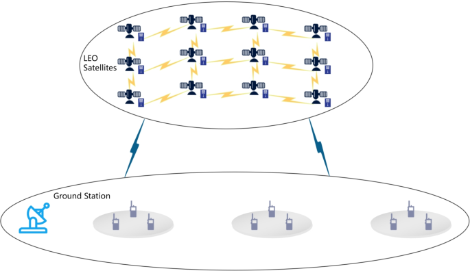
Satellite edge computing network architecture.
The main notations used in this paper are summarized in Table 1.
Table 1 List of main notations.Satellite network topology model
The network topology model represents satellites as nodes and inter-satellite links as edges32. The positions and connections of satellite nodes change periodically. In this paper, the satellite network topology can be characterized as shown in Equation (1).
$$\begin{aligned} G=\left( V,E,W_V\left( t\right) ,W_E\left( t\right) \right) . \end{aligned}$$
(1)
Where \(V=(V_1,V_2,\cdots ,V_n)\) represents the set of satellite nodes, and \(E=(e_{11},e_{12}, \cdots , e_{nn})\) characterizes the links, denoting the connectivity between all satellites. \(W_V(t)=\left\{ w_{v_i}\left( t\right) | v_i\in V\right\}\) denotes the weight attributes of the nodes at moment t, such as resource type and resource capacity. Similarly, \(W_E(t)=\left\{ w_{e_{ij}}\left( t\right) | e_{ij}\in E\right\}\) represents the weight attributes of the links at time t. The connection states of inter-satellite links and their weights vary over time and can be effectively represented by a dynamic adjacency matrix:
$$\begin{aligned} W_E\left( t\right) =\left[ \begin{matrix}e_{11}\left( t\right) & \cdots & e_{1n}\left( t\right) \\ \vdots & \ddots & \vdots \\ e_{n1}\left( t\right) & \cdots & e_{nn}\left( t\right) \\ \end{matrix}\right] . \end{aligned}$$
(2)
Where \(e_{ij}\left( t\right)\) represents the link resources between satellite node i and satellite node j at time t.
Unlike terrestrial network models, satellite networks are dynamic and their topology undergoes periodic changes over time. To address this challenge, time slicing is employed to divide the satellite network into discrete time slots, as illustrated in Fig. 2. Within each time slot, the satellite network topology is treated as static, allowing task offloading to be performed more effectively. This approach significantly reduces the complexity of solving the task offloading problem in satellite networks.
Fig. 2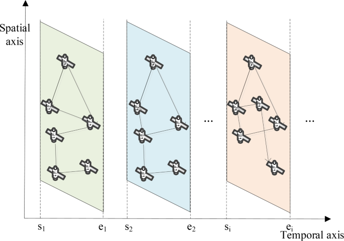
A dynamic topology analysis method based on time slicing.
Resource model
Satellite resources consist of computing, storage, and communication resources. To address the task offloading problem within a single time slice in a satellite edge computing network, it is assumed that the end user is covered by n edge computing satellite (ECS) nodes during time slice t. The set of satellite nodes is represented as:
$$\begin{aligned} {ECS}_t=\left( V_1,V_2,\cdots ,V_n\right) . \end{aligned}$$
(3)
Each satellite node is defined by a five-tuple that represents its heterogeneous resources:
$$\begin{aligned} V_i=\left( ID,f_c,R_c,R_s,R_L\right) . \end{aligned}$$
(4)
Here, ID is the unique identification of the resource, \(f_c\) denotes the computing speed of the satellite node, characterized by its CPU frequency, \(R_c\) indicates the computing resource capacity of the satellite node, \(R_s\) represents the storage resource capacity of the satellite node, and \(R_L\) describes the connections between different nodes, which can be expressed as a matrix:
$$\begin{aligned} R_L^{n\bullet n}=\left[ \begin{matrix}e_{11}& \cdots & e_{1n}\\ \vdots & \ddots & \vdots \\ e_{n1}& \cdots & e_{nn}\\ \end{matrix}\right] . \end{aligned}$$
(5)
Where \(e_{ij}\) is the link bandwidth resource between satellite node i and satellite node j in the current time slot. When \(i=j, e_{ij}=0\).
Task model
To effectively implement the task offloading strategy, it is essential to model large-scale task offloading requests in a reasonable manner33. Assume that a sequence of task requests is generated by m terminals, where each task is non-splitable:
$$\begin{aligned} Tasks=\left\{ T_1,T_2,\cdots ,T_m\right\} . \end{aligned}$$
(6)
Each task model is represented by a seven-tuple34:
$$\begin{aligned} T_i=\left\{ P,Data,T_C,T_S,T_L,T_{start},T_{dl}\right\} . \end{aligned}$$
(7)
Here, P represents the task priority, which is determined by the task type and is ranked as shown in Table 2. Data refers to the data size of the task. \(T_C\) denotes the computational resources required for the task, expressed as the number of processing cycles needed by the satellite CPUs. \(T_S\) represents the storage resources required for the task, where \(T_L\) indicates the link resources needed. \(T_{start}\) specifies the start time of the task, and \(T_{dl}\) represents the maximum latency the task can tolerate.
Computation offloading model
In task offloading decisions, the objective is to assign tasks to appropriate satellite nodes. Before selecting a satellite node, it is essential to consider the latency caused by task execution on each ECS node35. Due to the relatively short distance between LEO satellites and the ground, the propagation distance of tasks from the terminal to the satellite node is minimal, and the propagation speed is nearly equal to the speed of light. As a result, the propagation latency is negligible, and only computation latency and transmission latency are considered.
-
1.
Computation latency
Computation latency refers to the time required by a satellite to process a given task. The computation latency for satellite j to process task i is expressed as:
$$\begin{aligned} T_{i,proc}^j=\frac{T_{C,i}}{f_{j,i}}+T_{i,que}. \end{aligned}$$
(8)
-
2.
Transmission latency
In this paper, we focus solely on the transmission latency of tasks from the terminal to the satellite node. The transmission delay for terminal i sending data to satellite j is denoted as:
$$\begin{aligned} T_{i,trans}=\frac{{Data}_i}{r_{T_i,V_j}^{uplink}}. \end{aligned}$$
(9)
Where \(r_{T_i,V_j}^{uplink}\) is the transmission rate of the sub-channel assigned to task i by satellite j. Therefore, the total processing latency of task i is
$$\begin{aligned} T_{i,total}=T_{i,proc}^j+T_{i,trans}^j. \end{aligned}$$
(10)
Task offloading constraints
Assume that there are \(Tasks=\left\{ T_1,T_2,\cdots ,T_m\right\}\) offloaded to satellite node j simultaneously.
-
1.
Resource node constraints
When offloading tasks, ECS nodes must have sufficient resources. For the terminal task request sequence defined by Equation (6), the following conditions must be satisfied for any satellite node j:
$$\begin{aligned} \left\{ \begin{array}{cc} \sum _{i=1}^{m} T_C^i \le R_C^J & \\ \sum _{i=1}^{m} T_S^i \le R_S^J & \end{array} \right. \end{aligned}$$
(11)
The total computational resources required to process all tasks on satellite node j must not exceed the node’s available computational capacity, and the total storage space occupied by all tasks must not surpass the node’s storage capacity.
-
2.
Link Bandwidth Constraints
The bandwidth required for transmissions over the link must not exceed the total available bandwidth of the link.
$$\begin{aligned} \left\{ \sum _{i=1}^{m} T_L^i \le R_L^J \right. \end{aligned}$$
(12)
-
3.
Response time constraints
For any computational task i, the response time must not exceed its specified maximum allowable latency.
$$\begin{aligned} T_{i,total}\le T_{dl}. \end{aligned}$$
(13)
-
4.
Satellite visible time constraints
Define the task decision time as \({ST}_i\). Within the time slice t, terminal tasks can only be offloaded to the ECS node currently covering the region. Once the time slice ends, the edge computing satellite cluster changes, rendering the current offloading decision invalid. This results in the failure of the task offloading process and requires a new decision to be made. Let the start and end times of the time slice be defined as \(\left\{ {begin}_t,{end}_t\right\}\):
$$\begin{aligned} {begin}_t\le {ST}_i\le {end}_t. \end{aligned}$$
(14)
Multi-objective optimization function
The overall system resource utilization, defined as the weighted sum of computational resource utilization, storage resource utilization, and link resource utilization, is expressed as:
$$\begin{aligned} Rate_{total}=\alpha Rate_C+\beta Rate_S+\gamma Rate_L. \end{aligned}$$
(15)
Where \(\alpha\), \(\beta\), and \(\gamma\) are the weights assigned to each type of resource,representing their respective influence on the overall resource utilization, with the condition that \(\alpha +\beta +\gamma =1\). \(Rate_C\), \(Rate_S\), and \(Rate_L\) denote the utilization rates of computational resources, storage resources, and link resources, respectively.
The load balancing degree, denoted as \(r_{lb}\), is a system-level metric quantifying the resource utilization uniformity across n nodes in distributed systems, with a range within [0,1], where \(r_{lb} \rightarrow 1\) indicates higher balance. The load balancing degree calculation is as follows:
$$\begin{aligned} r_{lb}= {\left\{ \begin{array}{ll} 1 & \text {if } \mu = 0 \\ \dfrac{\mu }{\mu + \delta } & \text {otherwise} \end{array}\right. } \end{aligned}$$
(16)
where \(\mu\) and \(\delta\) can be calculated as follows:
$$\begin{aligned} \mu = E_{rate}=\dfrac{1}{n}\sum _{i=1}^{n}Rate_{total}^i \ \end{aligned}$$
(17)
$$\begin{aligned} \delta = \sqrt{\frac{1}{n} \sum _{i=1}^{n} \left( {Rate}_{{total}}^{i} – \mu \right) ^{2}} \end{aligned}$$
(18)
when \(\mu =0\) indicates that the system is in an idle state, with no active tasks being processed.
The goal of task offloading is to optimize the processing latency of all tasks, improve the task completion rate, and enhance resource utilization and load balancing within the satellite cluster, all while maintaining the quality of service for users. This approach ensures efficient resource allocation and prevents satellite nodes from becoming overloaded. The optimization problem is formulated as follows:
$$\begin{aligned} \left\{ \begin{array}{ll} {Min\ T}_{i,total} \\ {Max\ Rate}_{total} \\ {Max\ r}_{lb} \end{array} \right. \end{aligned}$$
(19)
To construct the reward function for multi-objective optimization, the task response latency is normalized as follows:
$$\begin{aligned} T_{i,total}^*=\frac{T_{i,total}}{T_{i,dl}-T_{i,start}}. \end{aligned}$$
(20)
Where \(T_{i,dl}\) denotes the maximum processing latency of task i offloading to different satellite nodes, and \(T_{i,start}\) is the start time of task i offloading. The normalized task latency \(T_{i,total}^*\in \left[ 0,1\right]\).
Based on the constraints outlined in Equations (11)-(14), the multi-objective optimization function in this paper is defined as follows:
$$\begin{aligned} Reward=-\alpha T_{i,total}^*+\beta Rate_{total}+\gamma r_{lb}. \end{aligned}$$
(21)
\(\alpha\), \(\beta\), and \(\gamma\) are weight coefficients, which can be set differently according to different types of application, and \(\alpha +\beta +\gamma =1\). In this paper, the coefficients are set as: \(\alpha\) = 0.4, \(\beta\) = 0.3, \(\gamma\) = 0.3.