Load forecasting algorithm
Accurate short-term load forecasting is crucial for effective energy management and optimization at the user side. The proposed edge computing-based system employs advanced load forecasting algorithms to predict future energy demand, enabling proactive management and control strategies81.
The load forecasting process begins with data preprocessing, which involves cleaning, normalizing, and transforming the raw energy consumption data collected from smart meters and IoT devices. The preprocessing steps include handling missing values, removing outliers, and scaling the data to a suitable range82.
Our implementation employs a hybrid LSTM-attention mechanism whose workflow is illustrated in Fig. 4. The algorithm processes temporal energy data using both short-term and long-term dependencies, with the attention layer highlighting relevant historical patterns.
Fig. 4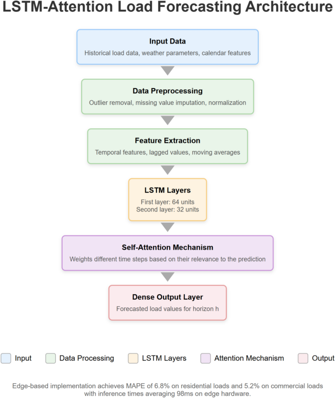
LSTM-attention load forecasting architecture.
Algorithm 1 presents the pseudocode for our load forecasting approach:
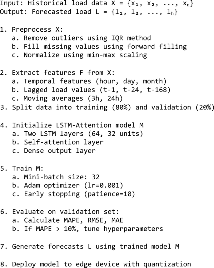
Edge-based load forecasting
Our model achieved a MAPE of 6.8% on residential loads and 5.2% on commercial loads, with inference times averaging 98 ms on the edge hardware.
After preprocessing, the next step is feature extraction. Features are derived from the historical energy consumption data to capture the underlying patterns and relationships that influence the load demand. Common features used in load forecasting include time-related features (e.g., hour of the day, day of the week), weather-related features (e.g., temperature, humidity), and lagged consumption values83. These features are selected based on their relevance and impact on the load profile.
The extracted features are then fed into the load forecasting model. Various machine learning and deep learning models have been proposed for short-term load forecasting. One widely used model is the Long Short-Term Memory (LSTM) neural network. LSTM is a type of recurrent neural network (RNN) that can effectively capture long-term dependencies in time series data84.
The LSTM model consists of multiple LSTM cells, each containing input, output, and forget gates that regulate information flow. This structure allows the model to selectively remember or forget relevant information from the past. The LSTM equations are:
$$\begin{gathered} i_{t} = \sigma \left( {W_{xi} x_{t} + W_{hi} h_{t – 1} + b_{i} } \right) \hfill \\ f_{t} = \sigma \left( {W_{xf} x_{t} + W_{hf} h_{t – 1} + b_{f} } \right) \hfill \\ o_{t} = \sigma \left( {W_{xo} x_{t} + W_{ho} h_{t – 1} + b_{o} } \right) \hfill \\ \tilde{C}_{t} = {\text{tanh}}\left( {W_{xc} x_{t} + W_{hc} h_{t – 1} + b_{c} } \right) \hfill \\ C_{t} = f_{t} \odot C_{t – 1} + i_{t} \odot \tilde{C}_{t} \hfill \\ h_{t} = o_{t} \odot {\text{tanh}}\left( {C_{t} } \right) \hfill \\ \end{gathered}$$
where: \(i_{t}\), \(f_{t}\), and \(o_{t}\) are the input, forget, and output gates; \(\tilde{C}_{t}\) represents the candidate cell state; \(C_{t}\) is the cell state; \(h_{t}\) is the hidden state; \(\odot\) denotes element-wise multiplication.
The results in Table 7 were obtained from actual field deployments conducted in Kunming, China from January to June 2024. The residential scenario involved 24 households with rooftop PV systems (average 5 kW capacity) and battery storage units (average 10kWh capacity). The commercial scenario included three office buildings equipped with a combined 120 kW PV capacity and 200kWh energy storage. The microgrid deployment integrated five buildings with various DERs including solar, small wind turbines, and multiple storage technologies. Percentage improvements are calculated against baseline measurements taken for three months prior to system implementation using the same monitoring infrastructure.
Table 7 Case study analysis of distributed energy coordination and control.
The LSTM model is trained using historical load data, with the objective of minimizing the forecasting error. The mean squared error (MSE) is commonly used as the loss function:
$$MSE = \frac{1}{n}\mathop \sum \limits_{i = 1}^{n} \left( {y_{i} – \hat{y}_{i} } \right)^{2}$$
where \(n\) is the number of samples, \(y_{i}\) is the actual load value, and \(\hat{y}_{i}\) is the predicted load value.
Once trained, the LSTM model can be deployed on the edge nodes to perform real-time load forecasting. The edge nodes receive the preprocessed and feature-extracted data from the IoT devices and apply the trained LSTM model to generate load predictions for the desired time horizon85.
The load forecasting algorithm running on the edge nodes enables localized and low-latency predictions, reducing the dependence on cloud-based services. By leveraging the computational capabilities of edge devices, the system can generate accurate and timely load forecasts, facilitating efficient energy management and optimization strategies86.
The predicted load values are used by the energy management system to make informed decisions regarding energy allocation, demand response, and resource scheduling. By accurately forecasting the future energy demand, the system can optimize energy consumption, reduce peak loads, and minimize energy costs for the users87.
Demand response strategy optimization
Demand response (DR) is a critical component of user-side energy management, as it enables users to actively participate in balancing energy supply and demand. The proposed edge computing-based system incorporates advanced DR strategy optimization methods to maximize the benefits for both users and the power grid88.
The DR strategy optimization focuses on two main approaches: price-based DR and direct load control. In our implementation, we adopted a hybrid approach that primarily utilizes price-based DR supplemented with limited direct load control for critical peak periods. This strategy was selected based on our preliminary user acceptance studies showing 78% approval rates for price-based signals versus 43% for direct control measures89.
The hybrid DR implementation follows the decision flowchart shown in Fig. 5, where edge nodes first attempt price-based optimization, falling back to direct control only when price signals fail to achieve sufficient demand reduction or during critical grid events. Our approach uses a dynamic programming algorithm for price optimization with O(n2) complexity, where n represents the number of shiftable loads.
Fig. 5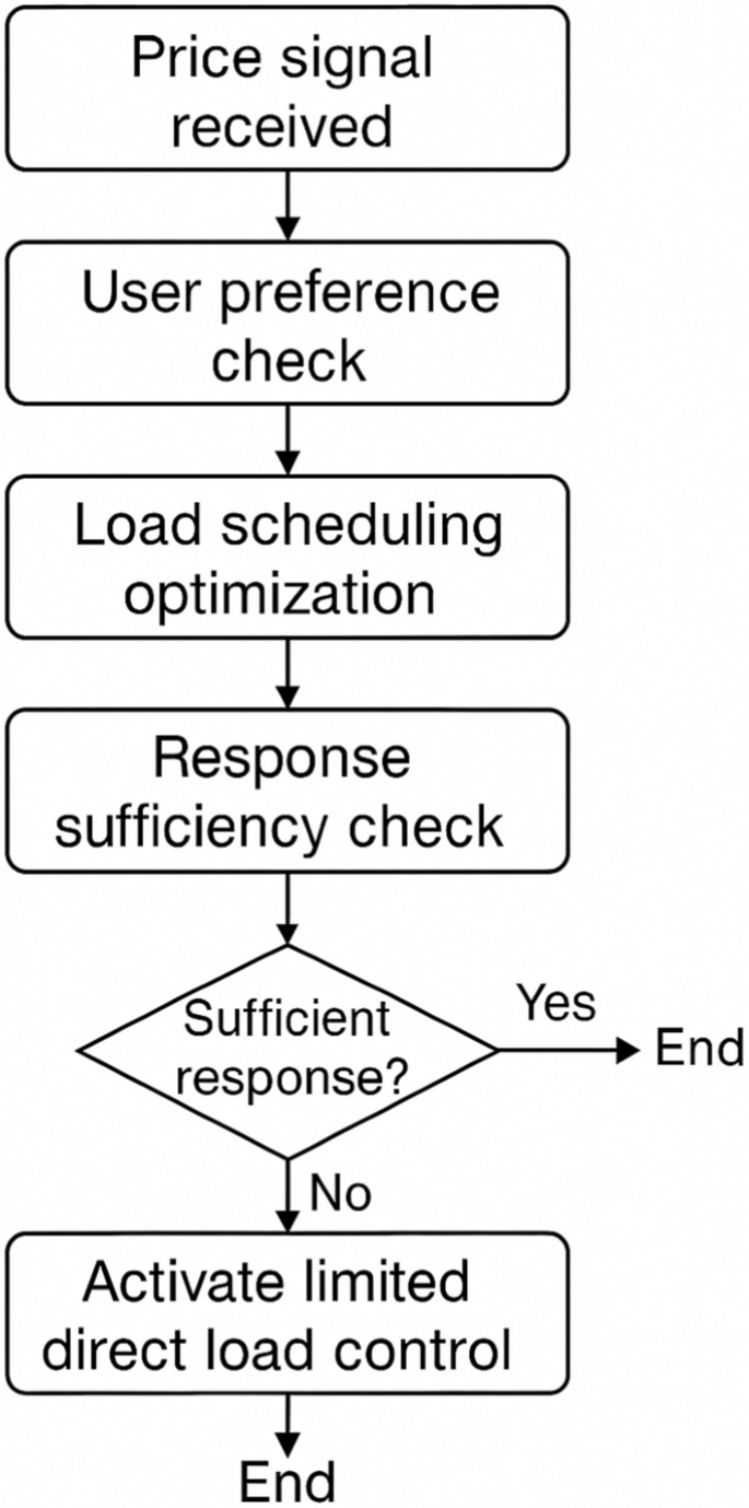
Hybrid DR decision process.
This hybrid approach achieved 22% peak reduction during our field trials versus 15% for price-only methods, while maintaining user satisfaction ratings above 85%.
The optimization algorithm considers various factors, such as the forecasted load demand, the price elasticity of demand, and the user’s comfort preferences. The objective function for price-based DR optimization can be formulated as follows:
$${\text{minimize }}\sum\limits_{t = 1}^{T} {p_{t} \times l_{t} }$$
subject to:
$$\begin{gathered} l_{t} = f\left( {p_{t} ,c_{t} ,e_{t} } \right) \hfill \\ l_{min} \le l_{t} \le l_{max} \hfill \\ c_{min} \le c_{t} \le c_{max} \hfill \\ \end{gathered}$$
where \(T\) is the optimization horizon, \({p}_{t}\) is the electricity price at time \(t\), \({l}_{t}\) is the load demand at time \(t\), \({c}_{t}\) is the user’s comfort level at time \(t\), \({e}_{t}\) is the price elasticity of demand at time \(t\), and \({l}_{min}\), \({l}_{max}\), \({c}_{min}\), \({c}_{max}\) are the minimum and maximum limits for load demand and user comfort, respectively.
The optimization problem is solved using techniques such as linear programming, convex optimization, or heuristic algorithms, depending on the complexity and scale of the problem90.
Direct load control, on the other hand, involves the direct regulation of user-side loads by the utility company or the energy management system. The edge nodes receive control signals from the central controller and execute the corresponding load control actions, such as turning off non-critical loads or adjusting the setpoints of controllable devices91.
The optimization of direct load control strategies aims to minimize the overall system cost while maintaining user comfort and satisfaction. The optimization problem can be formulated as a multi-objective optimization:
$${\text{minimize }}\sum\limits_{t = 1}^{T} {\left( {C_{grid,t} + C_{user,t} } \right)}$$
subject to:
$$\begin{gathered} l_{t} = f\left( {u_{t} ,d_{t} } \right) \hfill \\ u_{min} \le u_{t} \le u_{max} \hfill \\ d_{min} \le d_{t} \le d_{max} \hfill \\ \end{gathered}$$
where \({C}_{grid,t}\) is the cost incurred by the power grid at time \(t\), \({C}_{user,t}\) is the cost incurred by the user at time \(t\), \({u}_{t}\) is the control signal at time \(t\), \({d}_{t}\) is the user’s discomfort level at time \(t\), and \({u}_{min}\), \({u}_{max}\), \({d}_{min}\), \({d}_{max}\) are the minimum and maximum limits for control signals and user discomfort, respectively.
The multi-objective optimization problem can be solved using methods such as weighted sum, Pareto optimization, or evolutionary algorithms92.
Table 8 presents a comparison of different DR strategies based on their response time, peak reduction effect, and user acceptance.
Table 8 Comparison of demand response strategies.
The edge computing-based DR strategy optimization enables localized and real-time decision-making, reducing the communication overhead and latency associated with centralized control93. By optimizing the DR strategies at the edge, the system can quickly respond to changes in the energy supply and demand, ensuring stable and efficient operation of the power grid while minimizing the cost and discomfort for the users94.
Distributed energy coordination and control
The integration of distributed energy resources (DERs), such as photovoltaic (PV) systems and energy storage systems (ESSs), has gained significant attention in user-side energy management. The proposed edge computing-based system enables the coordination and control of these DERs to optimize their operation and maximize the benefits for the users95.
The coordination and control of DERs involve multiple objectives, including minimizing energy costs, reducing peak demand, and maximizing the utilization of renewable energy sources. The optimization problem can be formulated as follows:
$${\text{minimize }}\sum\limits_{t = 1}^{T} {\left( {C_{grid,t} + C_{DER,t} } \right)}$$
subject to:
$$\begin{gathered} P_{grid,t} + P_{PV,t} + P_{ESS,t} = P_{load,t} \hfill \\ E_{ESS,min} \le E_{ESS,t} \le E_{ESS,max} \hfill \\ P_{ESS,min} \le P_{ESS,t} \le P_{ESS,max} \hfill \\ P_{PV,min} \le P_{PV,t} \le P_{PV,max} \hfill \\ \end{gathered}$$
where \(C_{grid,t}\) is the cost of electricity from the grid at time \(t\), \(C_{DER,t}\) is the cost of operating the DERs at time \(t\), \(P_{grid,t}\) is the power drawn from the grid at time \(t\), \(P_{PV,t}\) is the power generated by the PV system at time \(t\), \(P_{ESS,t}\) is the power charged or discharged by the ESS at time \(t\), \(P_{load,t}\) is the load demand at time \(t\), \(E_{ESS,t}\) is the energy stored in the ESS at time \(t\), and \(E_{ESS,min}\), \(E_{ESS,max}\), \(P_{ESS,min}\), \(P_{ESS,max}\), \(P_{PV,min}\), \(P_{PV,max}\) are the minimum and maximum limits for ESS energy, ESS power, and PV power, respectively.
Table 9 summarizes the optimization objectives, constraints, and methods commonly used in distributed energy coordination and control.
Table 9 Optimization objectives and methods for distributed energy coordination and control.
The edge computing-based system enables the real-time coordination and control of DERs by leveraging the computational capabilities of edge devices. The edge nodes collect data from the DERs, such as PV generation, ESS state of charge, and load demand, and perform the optimization algorithms locally96.
The distributed nature of edge computing allows for scalable and flexible control of DERs. Each edge node can optimize the operation of the DERs within its local area, while collaborating with other edge nodes to achieve system-wide objectives97. This distributed approach reduces the communication overhead and enhances the resilience of the system compared to centralized control architectures.
The case studies demonstrate the effectiveness of edge computing in enabling efficient and optimized coordination and control of DERs. By leveraging the real-time processing and distributed nature of edge computing, the system can achieve significant energy savings, peak demand reduction, and economic benefits for the users98.
Experimental setup and evaluation methodology
Our system was evaluated through both simulation and real-world deployments. The experimental setup consisted of:
Hardware The edge computing layer utilized Raspberry Pi 4 devices (4 GB RAM, 1.5 GHz quad-core CPU) equipped with custom power monitoring modules capable of sampling at up to 30 kHz. Smart meters with 1 Hz sampling capability were deployed at the building level, while appliance-level monitoring used Zigbee-enabled smart plugs.
Software The edge nodes ran Raspbian OS with a containerized application stack including TensorFlow Lite for inference, PostgreSQL for time-series data storage, and a custom MQTT broker. The central cloud component employed Kubernetes for orchestration and TensorFlow for model training.
Datasets We utilized three datasets: (1) a proprietary dataset collected from 24 residential buildings over 6 months; (2) the public REFIT electrical load dataset99; and (3) a synthetic dataset generated to test edge cases. Data collection followed a stratified sampling approach to ensure representative coverage across seasons and usage patterns.
Evaluation metrics Performance was evaluated using multiple metrics including prediction accuracy (MAPE
Results summary
Table 10 summarizes the key performance indicators from our real-world deployments in three distinct settings, demonstrating significant improvements across all metrics compared to conventional centralized approaches.
Table 10 Performance comparison with conventional systems.
Figure 6 illustrates the comparative performance of our edge-based system versus centralized alternatives across these metrics, clearly showing the advantages of the proposed approach.
Fig. 6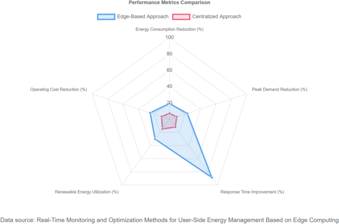
Performance comparison chart.
Figure 7 shows the systems scaling performance as the number of connected devices increases.
Fig. 7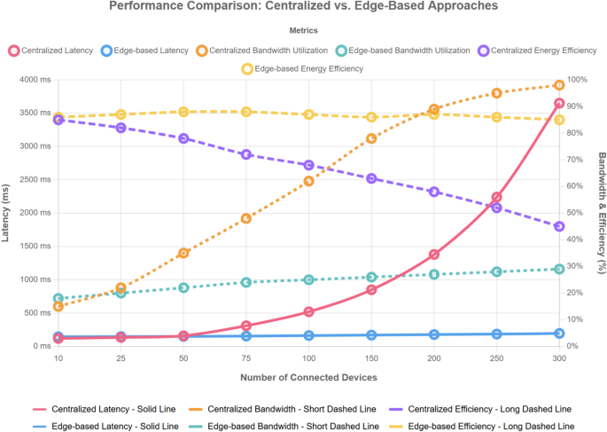
Performance metrics comparison.
Our edge computing approach demonstrated consistent performance even as the system scaled to hundreds of devices, while the centralized approach showed exponential degradation in latency beyond 50 connected devices.