Pure-state model for resonance fluorescence and its predictions
Figure 1a depicts the spontaneous emission model. A monochromatic laser coherently drives a TLE, e.g., a QD in a micropillar cavity11. Parameters ν, hν and TL are the laser’s frequency, photon energy and coherence time, respectively. The TLE’s excited state \(\left\vert e\right\rangle\) has a lifetime of T1, and a dephasing time of T2 (T2 ≤ 2T1). According to the optical Bloch equations, the TLE population reaches a steady state after ~ T1 time under steady continuous optical excitation4. Fundamentally, the TLE or its emission separately is in a mixed state. However, treating them jointly, it is possible, as derived in Section I, Supplementary Information, to use a pure-state description:
$${\left\vert \psi \right\rangle }_{t}=\sqrt{{p}_{0}}{\left\vert 0\right\rangle }_{t}{\left\vert g\right\rangle }_{t}+\sqrt{{p}_{1}}{e}^{-{{{\bf{i}}}}2\pi \nu t}\frac{{\left\vert 0\right\rangle }_{t}{\left\vert e\right\rangle }_{t}+{\left\vert 1\right\rangle }_{t}{\left\vert g\right\rangle }_{t}}{\sqrt{2}},$$
(1)
where \(\sqrt{{p}_{0}}\) and \(\sqrt{{p}_{1}}\) represent the magnitudes of the quantum probability amplitudes (p0 + p1 = 1). Here, \({\left\vert 0\right\rangle }_{t}{\left\vert e\right\rangle }_{t}\) means the TLE occupying its excited state has not spontaneously emitted at time t, while \({\left\vert 1\right\rangle }_{t}{\left\vert g\right\rangle }_{t}\) indicates emission of a photon has just taken place with the TLE having returned to its ground state \({\left\vert g\right\rangle }_{t}\). States \({\left\vert 0\right\rangle }_{t}{\left\vert e\right\rangle }_{t}\) and \({\left\vert 1\right\rangle }_{t}{\left\vert g\right\rangle }_{t}\) are connected only via spontaneous emission, and \({\left\vert 1\right\rangle }_{t}\) represents a spontaneously emitted photon at t contributing to the RF. By definition, \({\left\vert 1\right\rangle }_{t}\) is a broadband photon with bandwidth governed by the TLE’s dephasing time T2. The state \(\frac{{\left\vert 0\right\rangle }_{t}{\left\vert e\right\rangle }_{t}+{\left\vert 1\right\rangle }_{t}{\left\vert g\right\rangle }_{t}}{\sqrt{2}}\) implies that, at any given instant of time, it is not possible to know whether spontaneous emission has taken place or the TLE remains at its excited state \(\left\vert e\right\rangle\) prior to detection of a photon. However, once an RF photon is detected, we know for sure that spontaneous emission had taken place and the TLE returned to its ground state \(\left\vert g\right\rangle\) at the corresponding instant of time. An immediate detection of a second photon is prevented because the TLE requires time to be repopulated. This leads naturally to photon anti-bunching.
Fig. 1: Resonance fluorescence (RF).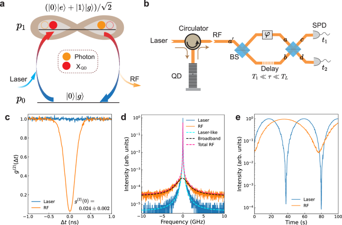
a Schematic for a two-level emitter (TLE) coherently driven by a continuous-wave laser into steady-state. Brackets \(\left\vert g\right\rangle\) and \(\left\vert e\right\rangle\) represent the ground and excited states of the TLE, while \(\left\vert 0\right\rangle\) and \(\left\vert 1\right\rangle\) mean 0 or 1 spontaneously emitted photon. Symbols p0 represents the population of the system ground state while p1 is the single-quanta population that is in a form of either the TLE staying at its excited state \((\left\vert 0\right\rangle \left\vert e\right\rangle )\)) or a fresh spontaneously emitted photon (\(\left\vert 1\right\rangle \left\vert g\right\rangle\)). b Schematic of the core experimental setup. The RF is collected in the same polarisation as the excitation laser. c Second-order correlation function g(2)(Δt) measurement traces. d High resolution spectra. e Interference fringes measured with the AMZI shown in (b). In this measurement we left the AMZI’s phase φ drift freely and recorded the count rate of the SPDs as a function of elapsed time. BS beam splitter, SPD single-photon detector.
Figure 1b shows an asymmetrical Mach-Zehnder interferometer (AMZI) suitable to evaluate the RF’s coherence. The AMZI’s delay (τ) is chosen to be much longer than the TLE relaxation time, but much shorter than the coherence time of the excitation laser, i.e., T1 ≪ τ ≪ TL, so as to ensure the steady-state, and phase-coherent, condition. The incoming RF signal from port \({a}^{{\prime} }\) is divided equally into two paths (a and b) by the first beam splitter and then recombine at the second one before detection at ports c and d by two single-photon detectors. When a photon is detected, it is not possible to distinguish whether the photon arose from the one emitted to an early time (t − τ) taking the long path or one emitted at a late time (t) taking the short path. Interference between the two indistinguishable paths occurs. As the coherence properties of an RF signal is unaffected by channel losses (see Section II, Supplementary Information), we can then use the pure-state of Eq. (1) as the input to analyse the interference outcome after the AMZI. The AMZI output state can be written as:
$$\left\vert {\Psi }_{{{{\rm{out}}}}}\right\rangle= {\left\vert {0}_{c}{0}_{d}\right\rangle }_{t}\left({p}_{0}\left\vert gg\right\rangle+\frac{\sqrt{{p}_{0}{p}_{1}}}{\sqrt{2}}\left\vert ge\right\rangle+\frac{\sqrt{{p}_{0}{p}_{1}}}{\sqrt{2}}\left\vert eg\right\rangle+\frac{{p}_{1}}{2}\left\vert ee\right\rangle \right)\\ +{\left\vert {1}_{c}{0}_{d}\right\rangle }_{t}\frac{\sqrt{{p}_{0}{p}_{1}}}{\sqrt{2}}\frac{1-{e}^{{{{\bf{i}}}}\varphi }}{\sqrt{2}}\left\vert gg\right\rangle+{\left\vert {1}_{c}{0}_{d}\right\rangle }_{t}\frac{{p}_{1}}{2\sqrt{2}}\left(\left\vert ge\right\rangle -{e}^{{{{\bf{i}}}}\varphi }\left\vert eg\right\rangle \right)-{\left\vert {2}_{c}{0}_{d}\right\rangle }_{t}{e}^{{{{\bf{i}}}}\varphi }\frac{{p}_{1}}{2\sqrt{2}}\left\vert gg\right\rangle \\ +{\left\vert {0}_{c}{1}_{d}\right\rangle }_{t}\frac{\sqrt{{p}_{0}{p}_{1}}}{\sqrt{2}}\frac{1+{e}^{{{{\bf{i}}}}\varphi }}{\sqrt{2}}\left\vert gg\right\rangle+{\left\vert {0}_{c}{1}_{d}\right\rangle }_{t}\frac{{p}_{1}}{2\sqrt{2}}\left(\left\vert ge\right\rangle+{e}^{{{{\bf{i}}}}\varphi }\left\vert eg\right\rangle \right)+{\left\vert {0}_{c}{2}_{d}\right\rangle }_{t}{e}^{{{{\bf{i}}}}\varphi }\frac{{p}_{1}}{2\sqrt{2}}\left\vert gg\right\rangle,$$
(2)
where φ denotes the AMZI phase delay and \(\left\vert xy\right\rangle\) (x, y = g, e) represents the TLE’s respective states corresponding to time bins t − τ and t. The first line contains no photons while the second and third lines represent photon outputs at ports c and d, respectively. Each output contains one phase-dependent term followed by two phase-independent ones. The phase-dependent term corresponds to the TLE’s transition \((\left\vert ge\right\rangle+\left\vert eg\right\rangle )/\sqrt{2}\to \left\vert gg\right\rangle\), which imparts the coherence to a superposition between two photon temporal modes: \(({\left\vert 0\right\rangle }_{t-\tau }{\left\vert 1\right\rangle }_{t}+{\left\vert 1\right\rangle }_{t-\tau }{\left\vert 0\right\rangle }_{t})/\sqrt{2}\). Varying the AMZI phase φ, this superposition will produce interference fringes with an amplitude of \(\frac{{p}_{0}{p}_{1}}{2}\), as opposed to the total output intensity of \(\frac{{p}_{1}}{2}\). Thus, the coherence level of the RF, quantified using the first-order correlation function g(1)(τ), has the form,
$${g}^{(1)}(\tau )={p}_{0}{e}^{-{{{\bf{i}}}}2\pi \nu \tau }.$$
(3)
Using Fourier transform, we infer that the RF consists of a spectrally sharp, laser-like (ll) part that inherits the linewidth of the driving laser and has a spectral weight of Ill/Itot = ∣g(1)(τ)∣ = p0 II–IV, Supplementary Information.
The reduction in coherence, by the amount of 1 − p0 or p1, is linked to the TLE’s transitions from the \(\left\vert ee\right\rangle\) state to \(\left\vert ge\right\rangle\), \(\left\vert eg\right\rangle\) or \(\left\vert gg\right\rangle\). As shown in Eq. (2), the first two transitions give rise to an incoherent single photon each while the last one produces a two-photon state. Transition \(\left\vert ee\right\rangle \to \left\vert ge\right\rangle\) (\(\left\vert ee\right\rangle \to \left\vert eg\right\rangle\)) emitted a photon into early (late) temporal mode but none at late (early) mode, so no two-path interference takes place. On the other hand, transition \(\left\vert ee\right\rangle \to \left\vert gg\right\rangle\) produces one photon into each mode, the interference of which causes coalescence and forms a photon-pair through Hong-Ou-Mandel (HOM) effect21. All these photons are incoherent, so they naturally display a bandwidth governed by the TLE’s transition and thus make up the broadband (bb) part, with a weight of Ibb/Itot = p1 in the RF spectrum.
In the absence of pure dephasing (T2 = 2T1), the relation of p0 and p1 with excitation power can readily be estimated through steady-state equilibrium. We define \(\bar{n}\) as the mean incident photon number over T1 duration11, and ηab as the TLE’s absorption efficiency under weak excitation limit. With absorption balancing out emission, we obtain \(\frac{\bar{n}}{{T}_{1}}\times {\eta }_{ab}\times (1-{p}_{1})=\frac{{p}_{1}}{2}\times \frac{1}{{T}_{1}}\), where the factor (1 − p1) on the left takes saturation into account while \(\frac{{p}_{1}}{2}\) on the right reflects on average only half of the excited state is in the matter form. We then have
$${p}_{0} =\frac{1}{1+2\bar{n}{\eta }_{ab}},\\ {p}_{1} =\frac{2\bar{n}{\eta }_{ab}}{1+2\bar{n}{\eta }_{ab}}.$$
(4)
These equations connect p0 and p1 directly to the single photon excitation level, and are applicable to both Heitler and Mollow excitation regimes. Since no assumption is made on the emitter type, Eq. (4) holds, under the condition T2 = 2T1, for all quantum two-level emitters, including a trapped atom8,10 or ion12, a molecule22, and a semiconductor QD13,14,15,16,23,24. The absorption efficiency ηab may vary drastically among emitters, but embedding an emitter into a cavity can enhance the light-matter interaction and could bring ηab close to unity. For a high-quality QD-micropillar device11,25,26, we expect \(| {g}^{(1)}(\tau )|={p}_{0}\simeq \frac{1}{1+2\bar{n}}\), which presents a unique test-point to our model.
Equation (2) yields another experimentally verifiable prediction. Looking at the third line of this equation, the laser-like component, though being dominant under weak excitation, can be completely eliminated through destructive interference by setting the AMZI phase to φ = π. Containing only the non-interfering single-photon term (\({\left\vert {0}_{c}{1}_{d}\right\rangle }_{t}\left(\left\vert ge\right\rangle -\left\vert eg\right\rangle \right)\)) and a photon-pair term (\({\left\vert {0}_{c}{2}_{d}\right\rangle }_{t}\left\vert gg\right\rangle\)), the output at port d closely resembles the result of passing a photonic state composed solely of vacuum and two-photon terms, \((1-\frac{{p}_{1}^{2}}{2})\left\vert 0\right\rangle \left\langle 0\right\vert+\frac{{p}_{1}^{2}}{2}\left\vert 2\right\rangle \left\langle 2\right\vert\), through a beam splitter. Naturally, the port d output with φ = π will exhibit excitation-flux-dependent super-bunching, as derived in Section V of the Supplementary Information:
$${g}^{(2)}(0)=\frac{1}{{p}_{1}^{2}}={\left(1+\frac{1}{2\bar{n}{\eta }_{ab}}\right)}^{2}.$$
(5)
At low pump limit (\(\bar{n}\to 0\)), the g(2)(0) value can theoretically be infinitely large. At the opposite limit (\(\bar{n}\to \infty\)), the RF loses all its first-order coherence according to Eq. (3) and the super-bunching disappears, i.e., g(2)(0) = 1. We remark that the predicted super-bunching is not observable with an incoherently pumped TLE.
Excitation-power dependence of the first-order coherence
To test, we use a QD-micropillar device11 featuring a quality factor of 9350 and a low cavity reflectivity of 0.015. It is kept in a closed-cycle cryostat and the QD’s neutral exciton is temperature-tuned into the cavity resonance at 13.6 K, emitting at 911.54 nm. The setup is schematically shown in Fig. 1b. We use a confocal microscope setup equipped with a tunable continuous-wave (CW) laser of 100 kHz linewidth as the excitation source and an optical circulator made of a polarising beam splitter and a quarter-wave plate for collecting the RF in the same polarisation of the driving laser11,27. The QD is characterised to have a Purcell enhanced lifetime of T1 = 67.2 ps (Fp ≃ 10), corresponding to a natural linewidth of γ∥/2π = 2.37 GHz, which is 15 times narrower than the cavity mode (κ/2π = 35 GHz). The RF is fed into a custom-built AMZI with a fixed delay of τ = 4.92 ns for interference before detection by single photon detectors. With additional apparatuses, the whole setup allows characterisations of high-resolution spectroscopy, auto-correlation function g(2)(Δt), the first-order correlation function g(1)(τ), and two-photon interference. All excitation fluxes used were strictly calibrated via the incident optical power (Pin) upon the sample surface using the relation of \(\bar{n}={P}_{in}{T}_{1}/h\nu\). Detailed description of the experimental setup can be found in “Methods”.
In the first experiment, we use a weak excitation flux of \(\bar{n}=0.0068\), corresponding to a Rabi frequency of Ω/2π = 210 MHz (~0.09γ∥). Figure 1c shows the auto-correlation function g(2)(Δt) for both the RF (orange line) and the laser (blue line). While the laser exhibits a flat g(2) because of its Poissonian statistics, the RF is strongly anti-bunched, with g(2)(0) = 0.024 ± 0.002, at the 0-delay over a time-scale of ~ T1, confirming that the QD scatters one photon at a time.
Figure 1d shows the RF frequency spectrum (orange line) measured with a scanning Fabry-Pérot interferometer (FPI). It is dominated by a sharp line that overlaps the laser spectrum (blue line) with a linewidth that is limited by the FPI resolution (20 MHz). The RF contains additionally a broadband pedestal whose amplitude is over 3 orders of magnitude weaker. The overall spectrum can be excellently fit with two Lorentzians of 20 MHz and 2.3 GHz linewidths, shown as cyan and black dashed lines, respectively. The bandwidth of the latter closely matches the TLE’s natural linewidth of γ∥/2π. Following the discussion surrounding Eq. (3), we attribute the sharp feature to the interference outcome of the RF signal passing through the FPI. The spectral weight of this laser-like peak can be measured using our AMZI (Fig. 1b), whose delay meets the steady-state condition T1 ≪ τ ≪ TL. An example result is shown in Fig. 1e, which gives a fringe visibility, or the laser-like fraction, of 0.94 for the RF. As comparison, the laser signal exhibits 0.9998 interference visibility.
Figure 2a shows high-resolution RF spectra under different excitation fluxes. As the flux increases, the broadband component increases its share of the total RF, and becomes considerably broadened when \(\bar{n}\) exceeds 0.25. It starts to develop into Mollow triplets at the few photon level as reported previously11. Nevertheless, the RF retains its single-photon characteristics for a flux up to \(\bar{n}=6.8\) when measured before the AMZI and without any spectral filtering, as demonstrated by the auto-correlation data (open squares) in Fig. 2b. At \(\bar{n}=6.8\), we measure g(2)(0) = 0.37, which is still below the limit (0.5) for a classical emitter.
Fig. 2: Coherence versus incident flux.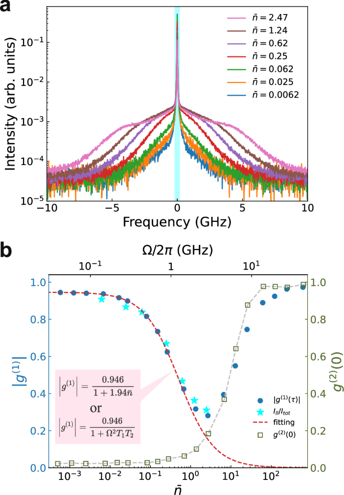
a High-resolution spectra; The cyan bar illustrates the laser-like spectral part. b ∣g(1)∣ (solid circles) measured with the AMZI and Ill /Itot (solid stars) extracted from data in (a), as well as g(2)(0) measured without any spectral filtering. The red dashed line is a fitting using either \(| {g}^{(1)}| \propto \frac{1}{1+x\bar{n}}\) with x = 1.94 or \(| {g}^{(1)}| \propto \frac{1}{1+{\Omega }^{2}{T}_{1}{T}_{2}}\) with T2 = 1.62T1.
The growing broadband component deteriorates the RF’s coherence. To quantify, we measure the interference visibility (∣g(1)∣) by passing the RF through the AMZI, with results shown as solid circles in Fig. 2b. This quantification method is equivalent to, and more precise than, calculating the area ratio of the laser-like peak to the total RF signal. The results from the latter method are shown as stars. At low fluxes (\(\bar{n} ), ∣g(1)∣ is plateaued at 0.946, rather than 1.0 as expected from Eq. (3). We attribute this discrepancy to photon distinguishability28, which could arise from phonon-scattering29,30,31 and QD environmental charge fluctuation32 as well as a small amount of laser mixed into the RF. As the flux increases until \(\bar{n}=3\), we observe a general trend of a decreasing visibility. For \(\bar{n} > 3.0\), the visibility reverses its downward trend and climbs up. In this regime, the RF signal starts to saturate11 while the laser background continues to rise, as evidenced by the accompanying rise in g(2)(0). At very strong fluxes (\(\bar{n} > 100\)), the laser background dominates because our setup collects the RF in the same polarisation of the driving laser, and thus the measured photon number statistics approaches Poissonian distribution, i.e., g(2)(0) ≈ 1.
We attribute the interference visibility drop in Fig. 2b to the increasing population (p1) of the QD’s exited state. Based on Eqs. (3) and (4), we obtain a near perfect fit, \(| {g}^{(1)}|=0.946/(1+x\bar{n})\) and x = 1.94, to the experimental data in the region where the RF signal remains dominant. The fitting is identical to the result (also shown as dashed line) by the traditional model3,13,26: \(| {g}^{(1)}| \propto \frac{1}{1+{\Omega }^{2}{T}_{1}{T}_{2}}\), where we use T2 = 1.62T1 and the Rabi frequencies extrapolated from the Mollow splittings measured under strong excitations. This is unsurprising because both models share the same theoretical foundation and \(\bar{n}\propto {\Omega }^{2}\) holds. However, our model gives a more direct link of the RF’s coherence to the excitation power, without the need for extracting the Rabi frequencies in order to achieve so. This experiment strongly supports our model and at the same time suggests an efficient input-coupling of our QD-micropillar device with ηab ≃ 0.97.
Photon super-bunching
In the next experiment (Fig. 3a), we use the AMZI to filter out the laser-like component by setting its phase to φ = π and then examine the super-bunching as expected in Eq. (4). As compared with a narrow-band filter6,7,8, this technique uses two-path, instead of multi-path, interference and thus the subsequent photon number statistics is easier to analyse. For the theoretical analysis, see Section V of Supplementary Information. Two AMZI-filtered spectra are shown in Fig. 3b. Each spectrum consists of a broadband signal with interference fringes of 203 MHz spacing corresponding to the AMZI’s delay (τ = 4.92 ns), while the laser-like component is rejected entirely. Subjecting the filtered RF to the auto-correlation measurement, we acquire a set of data shown in Fig. 3c. We observe super-bunching at 0-delay with g(2)(0) = 168.9 at the lowest flux of \(\bar{n}=0.0062\). At Δt = ± τ, interference between three temporal modes happens. Theoretically, \({g}^{(2)}(\pm \tau )\approx \frac{1}{4}{g}^{(2)}(0)\) under such incident flux. To compare, we have measured an average value of 47.6 for g(2)( ± τ), amounting to 0.282 of the corresponding g(2)(0) value.
Fig. 3: Correlation of the AMZI-filtered RF.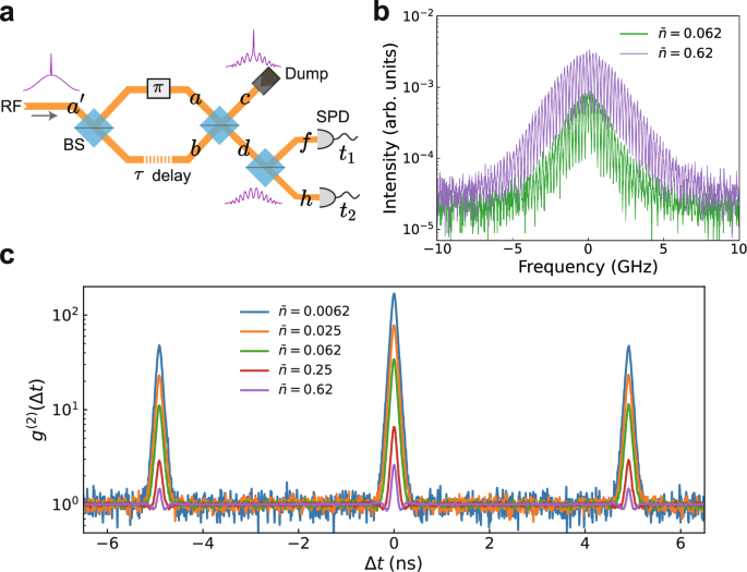
a Experimental setup; The AMZI is set to have a π phase so that the laser-like RF component is dumped at port c; The filtered RF at port d contains only the broadband component, and is fed into a HBT setup. b Filtered RF spectra; c Second-order correlation functions measured for various excitation fluxes.
We attribute the observed super-bunching to a combined effect of two-photon interference and the RF’s first-order destructive interference. The former generates two-photon states contributing to the 0-delay coincidences, while the latter reduces the photon intensity in the AMZI output port and thus suppresses the coincidence baseline. Setting φ = π maximises the level of super-bunching, but g(2)(0) can be tuned continuously down to anti-bunching through the AMZI phase. Details about AMZI phase stabilisation and measurements for other characteristic phases are shown in “Methods”.
As the excitation flux increases, we expect the RF’s first-order coherence to reduce and so will the level of super-bunching. Figure 3c shows the excitation flux dependence of the auto-correlation, which is in qualitative agreement with the theoretical prediction of Eq. (4). At \(\bar{n}=0.62\), we deduce p1 = 0.546 using the empirical relation of \({p}_{1}=1.94\bar{n}/(1+1.94\bar{n})\) and thus expect a photon bunching value of 3.35. Experimentally, we obtain g(2)(0) = 2.6, which is in fair agreement with the expected value. The discrepancy could arise from the increased laser background as well as finite photon indistinguishability28.
Phase-dependent two-photon interference
Finally, we perform phase-dependent two-photon interference experiment with the setup shown in Fig. 1b, and summarise the results in Fig. 4a with observations: (1) The coincidence baseline is phase-dependent, while the gap between traces shrinks as the excitation power increases; (2) Strong anti-bunching at Δt = 0 for all excitation fluxes and phase values; (3) Features at Δt = ±4.92 ns, caused by the AMZI’s delay τ, can exhibit as peaks or dips depending on both the excitation power and the phase delay. We note that observation (3) is strikingly different from incoherently excited quantum emitters26,33, where the side features always display as dips with depth limited to 0.75.
Fig. 4: Phase-dependent two-photon interference.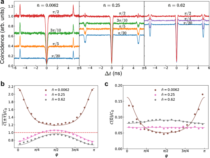
a Cross-correlation traces measured with the setup shown in Fig. 1b for three different excitation intensities: \(\bar{n}=0.0062\) (left), 0.25 (middle) and 0.62 (right panel). b Measured (solid symbols) and theoretical (solid lines) coincidence probabilities at Δt = ±τ delays, normalised to the coincidence baseline (dashed line). We use \(\overline{{{{\mathcal{C}}}}(\pm \tau )}=\frac{1}{2}\left({{{\mathcal{C}}}}(+\tau )+{{{\mathcal{C}}}}(-\tau )\right)\). c Normalised experimental (solid symbols) and theoretical (solid lines) coincidence probabilities at Δt = 0. Experimental data in b and c are extracted from data in (a). The theoretical results are fitted using maximum likelihood estimation. Fitted parameters \(\{{p}_{0},{p}_{1},{p}_{2};{M}^{{\prime} }\}\) corresponding to different excitation fluxes \(\bar{n}=0.0062,0.25,0.62\) are {0.98, 0.023, 8.0 × 10⁻⁶; 0.96}, {0.69, 0.30, 2.2 × 10⁻³; 0.94} and {0.49, 0.50, 8.0 × 10⁻³; 0.92}, respectively. A fixed value of M = 0.89, extracted from the plateaued ∣g(1)∣ = 0.946 shown in Fig. 2b through M = ∣g(1)∣2, is used for photon indistinguishability.
To understand the two-photon interference results, we approximate the RF output as a superposition of photon-number states: \({\left\vert {\psi }_{ph}\right\rangle }_{t}=\sqrt{{p}_{0}}{\left\vert 0\right\rangle }_{t}+\sqrt{{p}_{1}}{\left\vert 1\right\rangle }_{t}+\sqrt{{p}_{2}}{\left\vert 2\right\rangle }_{t}\) with a small two-photon probability \({p}_{2} \, \ll \, {p}_{1}^{2}/2\) and derive the coincidence probabilities as detailed in Section VI of Supplementary Information. We reproduce the main results below.
$${{{\mathcal{C}}}}(0)=\frac{{p}_{2}}{4}\left(1-{p}_{0}M\cos 2\varphi \right)+\frac{{p}_{1}^{2}+4{p}_{1}{p}_{2}+4{p}_{2}^{2}}{8}(1-{M}^{{\prime} }),$$
(6)
$${{{\mathcal{C}}}}(\pm \tau )=\frac{{p}_{1}^{2}}{16}(3-2{p}_{0}M\cos 2\varphi ),$$
(7)
$${{{{\mathcal{C}}}}}_{0}=\frac{{p}_{1}^{2}}{4}\left(1-{p}_{0}^{2}M{\cos }^{2}\varphi \right),$$
(8)
where M represents indistinguishability of the RF photons while \({M}^{{\prime} }\) is the post-selective two-photon interference visibility with detector jitter taken into account34. \({{{\mathcal{C}}}}(\Delta t)\) represents the coincidence probability at time interval Δt while C0 is the baseline coincidence. Equations (6)–(8) show all coincidence probabilities are phase-dependent. \({{{{\mathcal{C}}}}}_{0}\) and \({{{\mathcal{C}}}}(\pm \tau )\)’s dependence arises from the first-order interference, while \({{{\mathcal{C}}}}(0)\) contains contributions from \({\left\vert 2\right\rangle }_{t}\) states as well as incomplete HOM interference between two RF photons emitted separately by the AMZI delay τ. Figure 4b, c plots the phase dependence of the theoretical (solid lines) and experimental (symbols) coincidence rates for Δt = ±τ and Δt = 0, normalised to the baseline coincidence. We use maximum likelihood estimation method to determine a realistic set of parameters for each excitation flux that provide the best fit to the data. The theoretical simulations are in excellent agreement with the experimental data for three incident fluxes and have also successfully reproduced the crossover between \({{{\mathcal{C}}}}(\pm \tau )\) and \({{{{\mathcal{C}}}}}_{0}\) for \(\bar{n}=0.25\).