NP-hardness results indicate that finding exact optima and even sufficiently good approximate optima for worst-case instances of many optimization problems is probably out of reach for polynomial-time algorithms both classical and quantum4. Nevertheless, there remain combinatorial optimization problems, such as the closest vector problem, for which there is a large gap between the best approximation achieved by a polynomial-time classical algorithm5 and the strongest complexity-theoretic inapproximability result6. When considering average-case complexity, such gaps become more prevalent, as few average-case inapproximability results are known. These gaps present a potential opportunity for quantum computers, namely achieving in polynomial time an approximation that requires superpolynomial time to achieve using known classical algorithms.
Quantum algorithms for combinatorial optimization have been the subject of intense research over the last three decades7,8,9,10,11,12,13, which has uncovered some evidence of a possible superpolynomial quantum speed-up for certain optimization problems14,15,16,17,18,19,20. Nevertheless, the problem of finding a superpolynomial quantum advantage for optimization is extremely challenging and remains largely open.
Here we propose a quantum algorithm for optimization that uses interference patterns as its main underlying principle. We call this algorithm decoded quantum interferometry (DQI). DQI uses a quantum Fourier transform to arrange that amplitudes interfere constructively on symbol strings for which the objective value is large, thereby enhancing the probability of obtaining good solutions upon measurement. Most previous approaches to quantum optimization have been Hamiltonian-based7,8, with a notable exception being the superpolynomial speed-up due to Chen, Liu and Zhandry16 for finding short lattice vectors, which uses Fourier transforms and can be seen as an ancestor of DQI. Whereas Hamiltonian-based quantum optimization methods are often regarded as exploiting the local structure of the optimization landscape (for example, tunnelling across barriers21), our approach instead exploits the sparsity that is routinely present in the Fourier spectrum of the objective functions for combinatorial optimization problems, and it can also exploit more elaborate structure in the spectrum if present.
Before presenting evidence that DQI can efficiently obtain approximate optima not achievable by known polynomial-time classical algorithms, we quickly illustrate the essence of the DQI algorithm by applying it to max-XORSAT. We use max-XORSAT as our first example because, although it is not the problem on which DQI has achieved its greatest success, it is the context in which DQI is simplest to explain.
Given an m × n matrix B with m > n, the max-XORSAT problem is to find an n-bit string x satisfying as many as possible of the m linear mod-2 equations Bx = v. As we are working modulo 2, we regard all entries of the matrix B and the vectors x and v as coming from the finite field \({{\mathbb{F}}}_{2}\). The max-XORSAT problem can be rephrased as maximizing the objective function
$$f({\bf{x}})=\mathop{\sum }\limits_{i=1}^{m}{(-1)}^{{v}_{i}+{{\bf{b}}}_{i}\cdot {\bf{x}}},$$
(1)
where bi is the ith row of B and vi is the ith entry of v. Thus, f(x) is the number of the m linear equations that are satisfied minus the number unsatisfied.
From equation (1), one can see that the Hadamard transform of f is extremely sparse: it has m non-zero amplitudes, which are on the strings b1, …, bm. The state \({\sum }_{{\bf{x}}\in {{\mathbb{F}}}_{2}^{n}}f({\bf{x}})| {\bf{x}}\rangle \) is, thus, easy to prepare. Simply prepare the superposition \({\sum }_{i=1}^{m}{(-1)}^{{v}_{i}}| {{\bf{b}}}_{i}\rangle \) and apply the quantum Hadamard transform. (Here, for simplicity, we have omitted normalization factors). Measuring the state \({\sum }_{{\bf{x}}\in {{\mathbb{F}}}_{2}^{n}}f({\bf{x}})| {\bf{x}}\rangle \) in the computational basis yields a biased sample, where a string x is obtained with probability proportional to f(x)2, which slightly enhances the likelihood of obtaining strings with a large objective value relative to uniform random sampling.
To obtain stronger enhancement, DQI prepares states of the form
$$| P(f)\rangle =\sum _{{\bf{x}}\in {{\mathbb{F}}}_{2}^{n}}P(f({\bf{x}}))| {\bf{x}}\rangle ,$$
(2)
where P is an appropriately normalized degree-ℓ polynomial. The Hadamard transform of such a state always takes the form
$$\mathop{\sum }\limits_{k=0}^{{\ell }}\frac{{w}_{k}}{\sqrt{\left(\begin{array}{c}m\\ k\end{array}\right)}}\sum _{\begin{array}{c}{\bf{y}}\in {{\mathbb{F}}}_{2}^{m}\\ | {\bf{y}}| =k\end{array}}{(-1)}^{{\bf{v}}\cdot {\bf{y}}}| {B}^{{\rm{T}}}{\bf{y}}\rangle ,$$
(3)
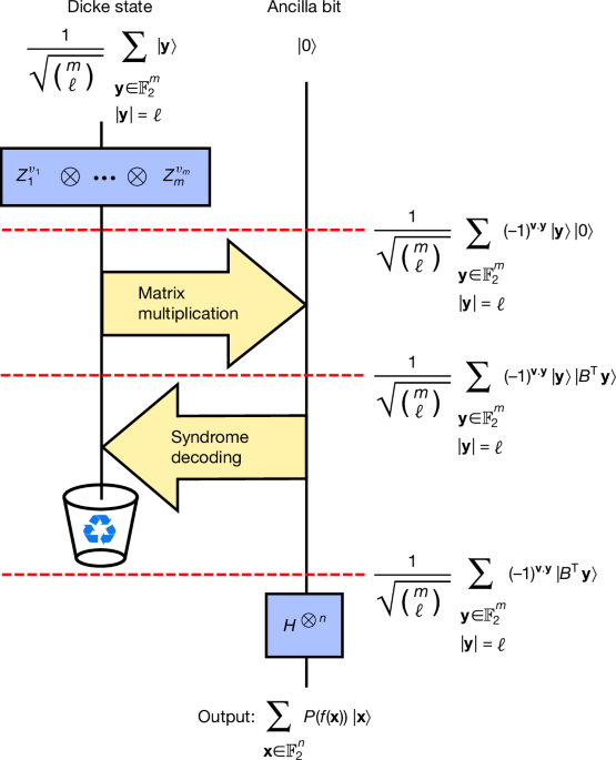
for some coefficients w0, …, wℓ. Here ∣y∣ denotes the Hamming weight of the bit string y. The DQI algorithm prepares |P(f)⟩ in five steps. The first step is to prepare the superposition \({\sum }_{k=0}^{{\ell }}{w}_{k}| {D}_{m,k}\rangle \), where
$$| {D}_{m,k}\rangle =\frac{1}{\sqrt{\left(\begin{array}{c}m\\ k\end{array}\right)}}\sum _{\begin{array}{c}{\bf{y}}\in {{\mathbb{F}}}_{2}^{m}\\ | {\bf{y}}| =k\end{array}}| {\bf{y}}\rangle $$
(4)
is the Dicke state of weight k. Preparing such superpositions over Dicke states can be done with \({\mathcal{O}}({m}^{2})\) quantum gates using the techniques in refs. 22,23. Second, the phase (−1)v⋅y is imposed by applying the product \({Z}_{1}^{{v}_{1}}\otimes \ldots \otimes {Z}_{m}^{{v}_{m}}\), where Zm is the Pauli-Z operator acting on the mth qubit. Third, the quantity BTy is computed into an ancilla register using a reversible circuit for matrix multiplication. This yields the state
$$\mathop{\sum }\limits_{k=0}^{{\ell }}\frac{{w}_{k}}{\sqrt{\left(\begin{array}{c}m\\ k\end{array}\right)}}\sum _{\begin{array}{c}{\bf{y}}\in {{\mathbb{F}}}_{2}^{m}\\ | {\bf{y}}| =k\end{array}}{(-1)}^{{\bf{v}}\cdot {\bf{y}}}| {\bf{y}}\rangle | {B}^{{\rm{T}}}{\bf{y}}\rangle .$$
(5)
The fourth step is to use the value BTy to infer y, which can then be subtracted from \(| {\bf{y}}\rangle \), thereby bringing it back to the all zeros state, which can be discarded. (This is known as ‘uncomputation’24). The fifth and final step is to apply a Hadamard transform to the remaining register, yielding |P(f)⟩. This sequence of steps is illustrated in Fig. 1.
Fig. 1: Schematic illustration of DQI.
As the initial Dicke state is of weight ℓ, the final polynomial P is of degree ℓ. Here, for simplicity, we take wℓ = 1 and wk = 0 for all k ≠ ℓ. Recycling icon adapted from FreeSVG (https://freesvg.org) under a CC0 1.0 Universal Public Domain licence.
The fourth step, in which |y⟩ is uncomputed, is not straightforward because B is a non-square matrix and, thus, inferring y from BTy is an underdetermined linear algebra problem. However, we also know that ∣y∣ ≤ ℓ. The problem of solving this underdetermined linear system with a Hamming weight constraint is precisely the syndrome decoding problem for the classical error-correcting code \({C}^{\perp }=\{{\bf{d}}\in {{\mathbb{F}}}_{2}^{m}:{B}^{{\rm{T}}}{\bf{d}}={\bf{0}}\}\) with up to ℓ errors.
In general, syndrome decoding is an NP-hard problem25. However, when B is very sparse or has certain kinds of algebraic structure, the decoding problem can be solved by polynomial-time classical algorithms even when ℓ is large (for example, linear in m). By solving this decoding problem using a reversible implementation of such a classical decoder, one uncomputes \(| {\bf{y}}\rangle \) in the first register. If the decoding algorithm requires T quantum gates, then the number of gates required to prepare |P(f)⟩ is \({\mathcal{O}}(T+{m}^{2})\).
Approximate solutions to the optimization problem are obtained by measuring |P(f)⟩ in the computational basis. The higher the degree of the polynomial in |P(f)⟩, the greater one can bias the measured bit strings towards solutions with a large objective value. However, this requires solving a harder decoding problem, as the maximum number of errors is equal to the degree of P. Next, we summarize how, by making an optimal choice of P and a judicious choice of decoder, DQI can be a powerful optimizer for some classes of problems.
Although DQI can be applied more broadly, the most general optimization problem that we apply DQI to in this paper is max-LINSAT, which we define as follows.
Definition 1
Let \({{\mathbb{F}}}_{p}\) be a finite field and let \(B\in {{\mathbb{F}}}_{p}^{m\times n}\). For each i = 1, …, m, let \({F}_{i}\subset {{\mathbb{F}}}_{p}\) be an arbitrary subset of \({{\mathbb{F}}}_{p}\), which yields a corresponding constraint \({\sum }_{j=1}^{n}{B}_{ij}{x}_{j}\in {F}_{i}\). The max-LINSAT problem is to find \({\bf{x}}\in {{\mathbb{F}}}_{p}^{n}\) satisfying as many as possible of these m constraints.
We focus primarily on the case that p has at most polynomially large magnitude and the subsets F1, …, Fm are given as explicit lists. The max-XORSAT problem is the special case where p = 2 and ∣Fi∣ = 1 for all i.
Consider a max-LINSAT instance where the sets F1, …, Fm each have size r. Let ⟨s⟩ be the expected number of constraints satisfied by the symbol string sampled in the final measurement of the DQI algorithm. Suppose we have a polynomial-time algorithm that can correct up to ℓ bit flip errors on codewords from the code \({C}^{\perp }=\{{\bf{d}}\in {{\mathbb{F}}}_{p}^{m}:{B}^{{\rm{T}}}{\bf{d}}={\bf{0}}\}\). Then, in polynomial time, DQI achieves the following approximate optimum to the max-LINSAT problem:
$$\frac{\langle s\rangle }{m}={\left(\sqrt{\frac{{\ell }}{m}\left(1-\frac{r}{p}\right)}+\sqrt{\frac{r}{p}\left(1-\frac{{\ell }}{m}\right)}\right)}^{2},$$
(6)
if r/p ≤ 1 − ℓ/m and ⟨s⟩/m = 1 otherwise. See Supplementary Theorem 1.1 for the precise statement for perfect decoding and Supplementary Theorem 7.1 for the analogous statement in the presence of decoding errors. This is achieved by a specific optimal choice of the coefficients w0, …, wℓ, which can be classically precomputed in polynomial time, as described in Supplementary Information section 6.
Note that r/p is the fraction of constraints that would be satisfied if the variables were assigned uniformly at random. When r/p = 1/2, equation (6) becomes the equation of a semicircle. Hence, we informally refer to equation (6) as the ‘semicircle law’.
From equation (6), any result on decoding a class of linear codes implies a corresponding result regarding the performance of DQI for solving a class of combinatorial optimization problems that are dual to these codes. This enables two new lines of research in quantum optimization. The first is to harvest the coding theory literature for rigorous theorems on the performance of decoders for various codes and obtain as corollaries guarantees on the approximation achieved by DQI for the corresponding optimization problems. The second is to perform computer experiments to determine the empirical performance of classical heuristic decoders, which, through equation (6), can be compared against the empirical performance of classical heuristic optimizers. In this manner, DQI can be benchmarked instance-by-instance against classical heuristics, even for optimization problems far too large to attempt on present-day quantum hardware. We next describe our results so far from each of these two lines of research.
We first use rigorous decoding guarantees to analyse the performance of DQI on the following problem.
Definition 2
Given integers n p − 1 with p prime, an instance of the optimal polynomial intersection (OPI) problem is as follows. Let F1, …, Fp−1 be subsets of the finite field \({{\mathbb{F}}}_{p}\). Find a polynomial \(Q\in {{\mathbb{F}}}_{p}[y]\) of degree at most n − 1 that maximizes fOPI(Q) = ∣{y ∈ {1, …, p − 1}: Q(y) ∈ Fy}∣, that is, that intersects as many of these subsets as possible.
An illustration of this problem is given in Fig. 2.
Fig. 2: Illustration of OPI problem.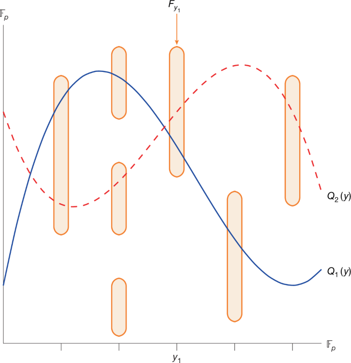
A stylized example of the OPI problem. For \({y}_{1}\in {{\mathbb{F}}}_{p}\), the orange set above the point y1 represents \({F}_{{y}_{1}}\). Both polynomials Q1(y) and Q2(y) represent solutions that have a large objective value, as they each intersect all but one set Fy.
In Supplementary Information section 2, we show that OPI is a special case of max-LINSAT over \({{\mathbb{F}}}_{p}\) with m = p − 1 constraints in which B is a Vandermonde matrix and, thus, C⊥ is a Reed–Solomon code. Syndrome decoding for Reed–Solomon codes can be solved in polynomial time out to half the distance of the code, for example, using the Berlekamp–Massey algorithm26. Consequently, in DQI we can take ℓ = ⌊(n + 1)/2⌋. For the regime where r/p and n/p are constants and p is taken asymptotically large, the fraction of satisfied constraints achieved by DQI using the Berlekamp–Massey decoder can be obtained by substituting ℓ/m = n/2p into equation (6).
OPI and special cases of it have been studied in several domains. In the coding theory literature, OPI is studied under the name ‘list-recovery’, and in the cryptography literature it is studied under the name ‘noisy polynomial reconstruction/interpolation’27,28. OPI can also be viewed as a generalization of the polynomial approximation problem, studied in refs. 29,30,31, in which each set Fi is a contiguous range of values in \({{\mathbb{F}}}_{p}\). In Supplementary Information section 8, we analyse the algorithms from these works in the literature and find that, for the parameter regime addressed by DQI, the best approximation achieved in polynomial time classically is 1/2 + n/2p using Prange’s algorithm. As shown in Fig. 3, for r/p = 1/2 and any fixed 0 n/p p. Classically, the only methods we are aware of to exceed the satisfaction fraction achieved by Prange’s algorithm are brute force search or slight refinements thereof, which have exponential runtime. Thus, DQI achieves a superpolynomial speed-up for this problem, assuming no polynomial-time algorithm is found that can match the satisfaction fraction that DQI achieves.
Fig. 3: Approximate optima for OPI.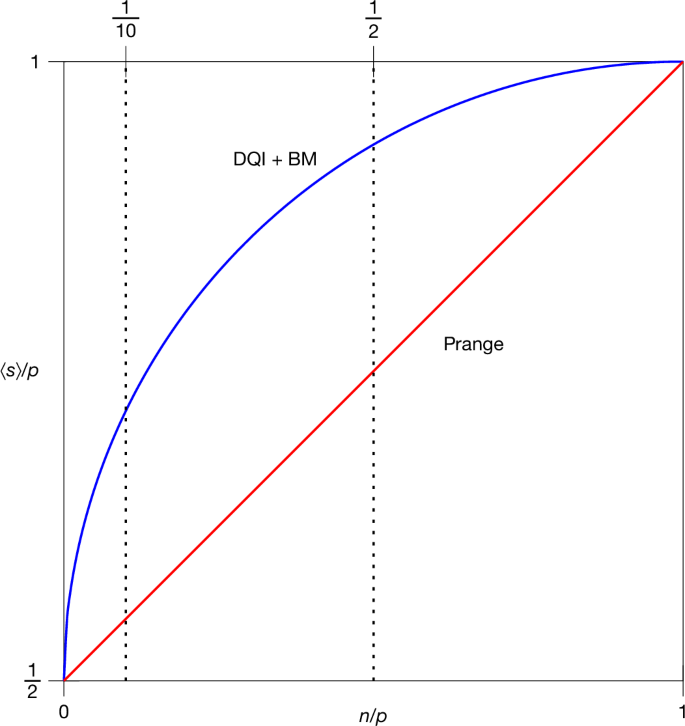
Plot of the expected fraction ⟨s⟩/p of satisfied constraints achieved by DQI with the Berlekamp–Massey decoder and by Prange’s algorithm for the OPI problem in the balanced case r/p = 1/2, as a function of the ratio of variables to constraints n/p. At n/p = 1/10, Prange’s algorithm satisfies a fraction 0.55 of the clauses whereas DQI satisfies \(\langle s\rangle /p=1/2+\sqrt{19}/20\approx 0.7179\). As a concrete challenge to the classical algorithms community, we propose matching or exceeding this value in polynomial time. In our concrete resource estimation, we consider n/p = 1/2, where OPI achieves \(\langle s\rangle /p=1/2+\sqrt{3}/4\approx 0.9330\) and Prange’s algorithm achieves 0.75. BM, Berlekamp–Massey decoder.
At present, there are no results directly showing that the OPI problem in the parameter regime that we consider is classically intractable under any standard complexity-theoretic or cryptographic assumptions. However, such results are known for certain limiting cases of the OPI problem, and we propose the task of extending these results to regimes more relevant to DQI for future research. The hardness of the special case of OPI when \(| \,{f}_{i}^{-1}(\,+1)| =1\), in a certain parameter regime, has been proposed as a cryptographic assumption in ref. 32, which has not been broken to our knowledge. Finding exact optima for OPI with \(| \,{f}_{i}^{-1}(\,+1)| =1\) can be cast as maximum-likelihood decoding for Reed–Solomon codes, which is known to be NP-hard33,34. Finding sufficiently good approximate optima is known to be as hard as discrete log35,36, but these hardness results do not match the parameter regime addressed by DQI.
As a concrete example, for n ≈ p/10 and r/p ≈ 1/2, the fraction of constraints satisfied by Prange’s algorithm is 0.55, whereas DQI achieves \(1/2+\sqrt{19}/20\approx 0.7179\). As a specific point of comparison, we challenge the algorithms community to beat this with a classical polynomial-time algorithm. Interestingly, for these parameters, one statistically expects that solutions satisfying all p − 1 constraints exist, but they apparently remain out of reach of polynomial-time algorithms both quantum and classical.
To find classically intractable instances of OPI solvable by DQI with minimal quantum resources, we find it is advantageous to choose n/p ≈ r/p ≈ 1/2. For these parameters, DQI achieves satisfaction fraction 0.933. As discussed in Supplementary Information section 13, achieving this using classical algorithms known to us has a prohibitive computational cost for p as small as 521. The dominant cost in DQI plus the Berlekamp–Massey decoder is the reversible implementation of the subroutine to find the shortest linear-feedback shift register used in the Berlekamp–Massey algorithm. Using Qualtran37, we find that at p = 521, the linear-feedback shift register can be found using approximately 1 × 10⁸ logical Toffoli gates and 9 × 10³ logical qubits.
We next use computer experiments to benchmark the performance of DQI against classical heuristics on average-case instances from certain families of max-XORSAT with sparse B. DQI reduces such problems to decoding problems on codes with sparse parity-check matrices. Such codes are known as low-density parity-check (LDPC) codes. Polynomial-time classical algorithms, such as belief propagation, can decode randomly sampled LDPC codes up to numbers of errors that nearly saturate information-theoretic limits3,38,39. This makes sparse max-XORSAT an enticing target for DQI. Although we use max-XORSAT as a convenient test bed for DQI, other commonly studied optimization problems, such as max-k-SAT, could be addressed similarly. Specifically, consider any binary optimization problem in which the objective function counts the number of satisfied constraints, where each constraint is a Boolean function of at most k variables. By taking the Hadamard transform of the objective function, one converts such a problem into an instance of weighted max-k-XORSAT, where the number of variables is unchanged and the number of constraints has been increased by at most a factor of 2k.
Although we are able to analyse the asymptotic average-case performance of DQI rigorously, we do not restrict the classical competition to algorithms with rigorous performance guarantees. Instead, we choose to set a high bar by also attempting to beat the empirical performance of classical heuristics that lack such guarantees.
Through careful tuning of sparsity patterns in B, we are able to find some families of sparse max-XORSAT instances for which DQI with standard belief-propagation decoding finds solutions satisfying a larger fraction of constraints than we are able to find using a comparable number of computational steps by any of the general-purpose classical optimization heuristics that we tried, which are listed in Table 1. However, unlike our OPI example, we do not put this forth as a potential example of superpolynomial quantum advantage. Rather, we are able to construct a tailored classical algorithm specialized to these instances, which, with 7 min of runtime, finds solutions where the fraction of constraints satisfied slightly beats DQI plus belief propagation (DQI + BP). As discussed in Supplementary Information section 9, our tailored heuristic is a variant of simulated annealing that assigns temperature-dependent weights to the terms in the cost function determined by how many variables they contain.
Table 1 Approximate optima for max-XORSAT
The comparison against simulated annealing is complicated because, as shown in Supplementary Information section 8.2, the fraction of clauses satisfied by simulated annealing increases as a function of the duration of the anneal. Thus, there is not a unique sharply defined number indicating the maximum satisfaction fraction reachable by simulated annealing. DQI reduces our sparsity-tuned max-XORSAT problem to an LDPC decoding problem, which our implementation of belief propagation solves in approximately 8 s on a single core, excluding the time used to load and parse the instance. Thus, a natural point of comparison is the result obtained by simulated annealing with a similar runtime. By running our optimized C++ implementation of simulated annealing for 8 s, we are only able to reach 0.764. If we allow the parallel execution of several anneals and increase our runtime allowance, we are able to eventually replicate the satisfaction fraction achieved by DQI + BP using simulated annealing. The shortest anneal that achieved this used five cores and ran for 73 h, which is five orders of magnitude longer than our belief-propagation decoder. Although this is dependent on the implementation details, we can take this ratio of runtimes as a rough indicator of the ratio of computational steps. In the context of DQI, the decoder would need to be implemented as a reversible circuit and subject to an overhead due to quantum error correction, so this should not be interpreted as an indicator of the quantum versus the classical runtime.