To illustrate this further, we now demonstrate how equation (4) leads to entanglement in a version of Feynman’s experiment. Two spherical mass distributions, each with total mass M and radius R, are prepared in a quantum superposition of two locations. This could be achieved by, for example, implementing matter-wave beam splitters6, manipulating potentials32 or exploiting internal degrees of freedom, such as quantum spins in Stern–Gerlach experiments5 (Fig. 3). Gravity is assumed to be the only interaction between the particles, and in the non-relativistic limit and describing matter within first quantization, it just acts as a quantum phase φij ≔ GM2t/(ħ dij) on each superposition branch5,6, where dij is the distance between the matter distributions in the branch labelled by i, j ∈ {L, R}, and GM2/dij is the Newtonian potential energy. With the superposition size Δx much greater than the smallest distance dRL, only the quantum phase φ ≔ φRL is significant, so that the systems are clearly entangled, with the entanglement depending solely on φ (refs. 5,6). By contrast, when Δx ≪ dRL, the relevant parameter for entanglement becomes essentially \(\overline{\varphi }:= \varphi \,\Delta {x}^{2}/{d}_{{\rm{RL}}}^{2}\) (ref. 33). To measure the entanglement, the superposed paths could be recombined and correlations sought between the interferometer outputs6 or internal degrees of freedom5.
Fig. 3: Visualization of a version of Feynman’s experiment.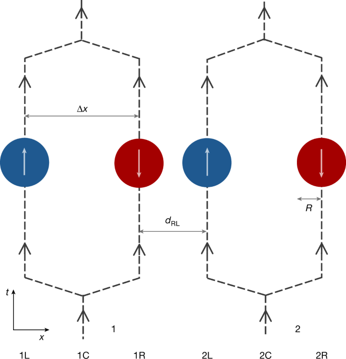
Two spherical mass distributions (1 and 2) of radius R are placed in quantum superpositions at two locations as N00N states, with blue and red denoting the components separated by Δx. After gravitationally interacting for a short time, the paths are recombined and entanglement is sought5,6. Although Stern–Gerlach interferometry with internal spins is illustrated5, alternative set-ups, such as parallel Mach–Zehnders, are also possible6. Here, Δx is depicted larger than the minimum separation dRL, but a general configuration can be implemented, including Δx ≪ dRL.
Quantum gravity
We now analyse this experiment using perturbative quantum gravity with a QFT description of matter. With electromagnetic interactions ignored, we take the initial state of the objects immediately after being placed in a quantum superposition as a product of N00N states:
$$\begin{array}{l}|\varPsi \rangle =\frac{1}{2}({|N\rangle }_{{\rm{1L}}}{|0\rangle }_{{\rm{1R}}}{|\uparrow \rangle }_{1}+{|0\rangle }_{{\rm{1L}}}{|N\rangle }_{{\rm{1R}}}{|\downarrow \rangle }_{1})\\ \qquad \otimes ({|N\rangle }_{{\rm{2L}}}{|0\rangle }_{{\rm{2R}}}{|\uparrow \rangle }_{2}+{|0\rangle }_{{\rm{2L}}}{|N\rangle }_{{\rm{2R}}}{|\downarrow \rangle }_{2}),\end{array}$$
(5)
where |N⟩κi is a product of N independent position states of matter particles obeying a complex scalar field34, with κ ∈ {1, 2} and i ∈ {L, R} labelling the position of the spherical objects (matching Fig. 3). N is the number of particles in the objects, such that M = mN, with m the mass of the particles. We also include possible internal spin states {|↑⟩, |↓⟩}, which could be used to generate the quantum superpositions.
After a time t, the state of the matter system in the Schrödinger picture is
$$| \varPsi (t)\rangle ={{\rm{e}}}^{{\rm{i}}{\widehat{H}}_{0}t/\hbar }\widehat{T}{{\rm{e}}}^{-({\rm{i}}/\hbar ){\int }_{0}^{t}{\rm{d}}\tau {\widehat{H}}_{{\rm{I}}}(\tau )}| \varPsi \rangle ,$$
(6)
where \(\widehat{T}\) is the time-ordering operator, τ is a dummy time variable, \({\widehat{H}}_{0}\) is the Hamiltonian of perturbative quantum gravity in the absence of matter–gravity interactions and \({\widehat{H}}_{{\rm{I}}}:= \exp ({\rm{i}}{\widehat{H}}_{0}t/\hbar ){\widehat{H}}_{{\rm{int}}}\,\exp (-{\rm{i}}{\widehat{H}}_{0}t/\hbar )\). Just before the superposition paths are bought back together, for example through reverse Stern–Gerlachs1,5, we can write
$$\begin{array}{l}|\,\varPsi (t)\rangle \propto {\alpha }_{{\rm{LL}}}{|N\rangle }_{{\rm{1L}}}{|N\rangle }_{{\rm{2L}}}+{\alpha }_{{\rm{LR}}}{|N\rangle }_{{\rm{1L}}}{|N\rangle }_{{\rm{2R}}}\\ \qquad \,+\,{\alpha }_{{\rm{RL}}}{|N\rangle }_{{\rm{1R}}}{|N\rangle }_{{\rm{2L}}}+{\alpha }_{{\rm{RR}}}{|N\rangle }_{{\rm{1R}}}{|N\rangle }_{{\rm{2R}}},\end{array}$$
(7)
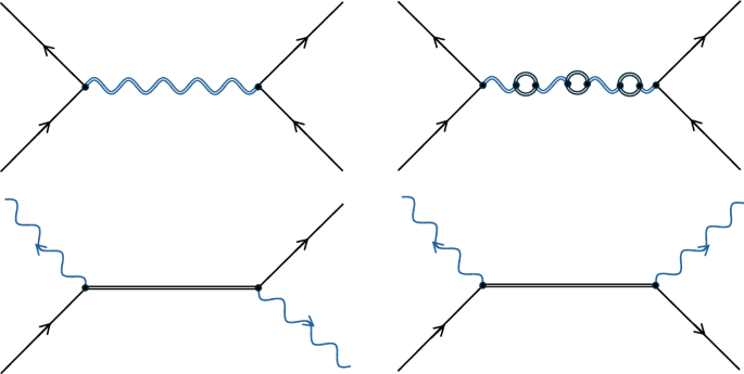
where \({\alpha }_{ij}\in {\mathbb{C}}\). We have now neglected any internal spin states and the vacuum states for simplicity. We can calculate the amplitudes αij by taking the inner product of equation (7) (and also equation (6)), with the basis states |N⟩1i |N⟩2j and expanding the time-ordered unitary operation in equation (6) as the Dyson series26,35. The amplitudes can then be written as a perturbative series with each term corresponding to that of the Dyson series: \({\alpha }_{ij}={\alpha }_{ij}^{(0)}+{\alpha }_{ij}^{(1)}+{\alpha }_{ij}^{(2)}+\cdots \,\). The first process where a virtual graviton is exchanged between the matter objects occurs at second order in the series and corresponds to the Feynman diagram in Fig. 1 (top left). The amplitude for this Feynman diagram, within the very good approximation ct ≫ dij (Methods), is
$$\frac{G{M}^{2}t}{\hbar {V}^{2}}\iint {{\rm{d}}}^{3}{\bf{x}}\,{{\rm{d}}}^{3}{\bf{y}}\frac{{\theta }_{1i}({\bf{x}}){\theta }_{2j}({\bf{y}})}{| {\bf{x}}-{\bf{y}}| }\equiv {\varphi }_{ij},$$
(8)
where θκi(x) ≔ θ(R − ∣x − Xκi∣) is the unit-step function defining the spherical shape of the matter distribution κ in branch i, Xκi is the coordinate for the centre of mass for the distributions and V ≔ 4πR3/3. The above amplitude directly contributes to \({\alpha }_{ij}^{(2)}\) such that, when Δx ≫ dRL, the \({\alpha }_{{\rm{RL}}}^{(2)}\) amplitude dominates over all others and equals iφ. Then, given that \({\alpha }_{ij}^{(0)}=1\) from the Dyson series and that \({\alpha }_{ij}^{(1)}\) contains no contractions for the gravitational field, we are left with αij ≈ 1 except for αRL ≈ 1 + iφ, which matches the first-quantized result to first order in the quantum phase \(\exp ({\rm{i}}\varphi )\). The full non-perturbative result is straightforwardly obtained by considering the form of the corresponding higher-order Feynman diagrams and extrapolating the result26.
Classical gravity
We now consider the above experiment within the context of classical gravity. The calculation follows the above but with the interaction Hamiltonian of equation (4) rather than equation (2). At second order in the Dyson series there are no non-vanishing Wick contractions corresponding to Feynman diagrams that contain quantum communication between the matter objects, and the diagram responsible for entanglement in quantum gravity, Fig. 1 (top left), becomes Fig. 2 (top middle). This diagram represents the two matter objects sitting in their combined classical gravitational field, with the amplitude just contributing a local relative quantum phase between the branches of each matter object, which does not lead to entanglement13. However, at fourth order in the series, a diagram appears where the matter distributions are connected quantum mechanically through virtual matter particles (Fig. 2, top right). Within the same approximations as in the quantum gravity case, the amplitude for the Feynman diagram is (Methods)
$${{\vartheta }}_{ij}:= \frac{{m}^{6}{t}^{2}{N}^{2}}{4{{\rm{\pi }}}^{2}{\hbar }^{6}{V}^{2}}{\left(i\int {{\rm{d}}}^{3}{\bf{x}}{{\rm{d}}}^{3}{\bf{y}}\frac{\varPhi ({\bf{x}})\varPhi ({\bf{y}}){\theta }_{1i}({\bf{x}}){\theta }_{2j}({\bf{y}})}{| {\bf{x}}-{\bf{y}}| }\right)}^{2},$$
(9)
where Φ(x) ≔ −c2h00(x)/2 is the total gravitational potential of the matter objects, and ϑij directly contributes to \({\alpha }_{ij}^{(4)}\) in equation (7). As we have a classical theory of gravity, Φ(x) is the same in each superposition branch, otherwise the Newtonian force would be in a quantum superposition. Certain works have considered gravity to be classical but still allow the field or Newtonian force to be in a quantum superposition36,37,38,39. Here, we keep to the notion that quantum superposition is a purely quantum-mechanical phenomena such that Φ(x) is not superposed in equation (9) and is not a quantum operator. However, despite this, equation (9) generically results in entanglement, as θ1i(x) and θ2i(x) are different for the different superposition paths and are connected through ∣x − y∣, such that \({\alpha }_{ij}^{(4)}\) is different for each superposition path, except for \({\alpha }_{{\rm{LL}}}^{(4)}={\alpha }_{{\rm{RR}}}^{(4)}\) from symmetry. We can understand this from the Feynman diagram in Fig. 2 (top right), where, unlike the gravitational potential, the virtual matter particles enter into a quantum superposition with the different mass states and the distance the virtual matter particles propagate is different in each branch, resulting in the spatial integrals in equation (9) being connected through ∣x − y∣.
As Φ(x) comes from a superposition of matter in equation (9), we must consider exactly how gravity is sourced by quantum matter in a fundamental theory of classical gravity. In the approach most considered40,41, Φ(x) in equation (9) is the sum of the average potentials of the superposition states of the two objects. In this case, ϑij is inversely proportional to dij such that, if Δx ≫ dRL, the RL amplitude dominates over all others and is ∣ϑRL∣ ≈ ϑ, where (Methods)
$$\sqrt{{\vartheta }}=\frac{6}{25}\frac{{G}^{2}{m}^{2}{M}^{3}Rt}{{\hbar }^{3}{d}_{{\rm{RL}}}}.$$
(10)
The state in equation (7) is then clearly entangled, because, just as in quantum gravity, αRL contains a contribution ϑ that is not in any of the other amplitudes αij. Furthermore, like quantum gravity33, the inverse scaling of ϑij with dij allows \(\overline{{\vartheta }}:= {\vartheta }\,\Delta {x}^{2}/{d}_{{\rm{RL}}}^{2}\) to be identified as the relevant parameter for entanglement when Δx ≪ dRL.