In silico validation of 16S rRNA gene metataxonomic analysisVaginal mock community and database selection
To select the most suitable database for this dataset, a comparison of different 16S rRNA gene taxonomic databases was conducted using an in silico-generated vaginal mock community. Following information from the literature23, the mock community was designed to represent the most common bacterial taxa found in vaginal samples across all CSTs. A total of 1,000 in silico 16S rRNA gene amplicons were simulated using Grinder (version 0.5.3)36 with its in silico PCR option, employing genomic DNA sequences from the selected taxa and standard full-length 16S rRNA primer sequences. Of the 11 taxa chosen initially, only 7 were successfully amplified under these simulation conditions; amplification failed for the strains Gardnerella vaginalis, Ureaplasma parvum ATCC 27815, Bifidobacterium breve, and Megasphaera paucivorans. The estimated relative abundances of the amplicons for each taxon are summarized in Table 2.
Table 2 Species present in in-silico mock community. All in silico amplicons are in an equal relative abundance of 12.5% in the mock community.
To mimic the error profile of Oxford Nanopore Technologies (ONT) long-read sequencing, we introduced errors into the in silico simulated amplicons using CuReSim-LoRM37, a simulator that generates realistic ONT-like read errors based on empirical models. The resulting reads constituted the final vaginal mock community. Considering the benchmarking performance of the Emu tool15, this method was selected for 16S taxonomic assignment. Three 16S rRNA databases were evaluated with this tool using the generated mock community: the Emu database, the SILVA database version available for Emu, and a GTDB database version adapted for Emu. Relative abundances obtained for the mock community at the genus level for each database are shown in Table 3 and graphically represented in Fig. 1. The estimated relative abundances from all databases were close to the expected values, with minor deviations attributable to simulated sequencing errors or taxonomic misassignments. Among the three databases, the Emu database demonstrated the highest concordance with expected abundances, showing relative abundances closest to the expected values, the lowest mean absolute error (0.0116), and misassigning only two genera.
Table 3 Relative genus abundances of in silico vaginal mock community estimated with different databases.Fig. 1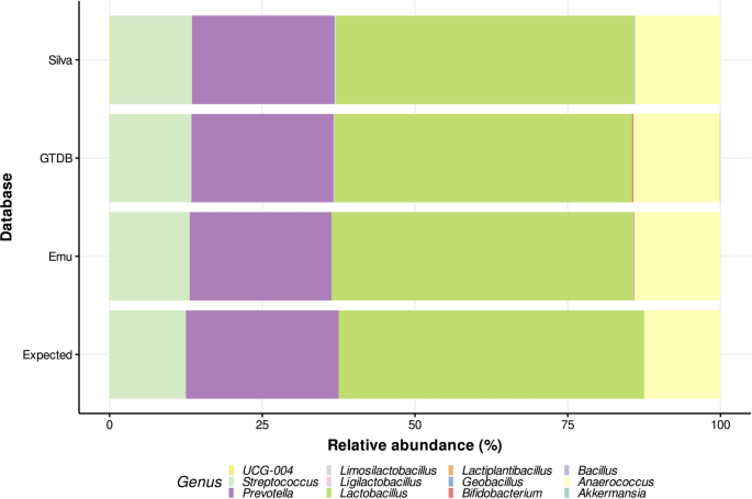
Relative abundance plot of the in silico vaginal mock community comparing the three databases used. Bars represent relative abundances estimated in the mock community with different databases using the Emu tool.
The same analysis was conducted at the species level for the three databases, with a summarized version of the results presented in Table 4. In all cases, the relative abundances closely align with the expected values; however, certain species are either underrepresented or overrepresented. For instance, Lactobacillus crispatus is consistently overrepresented across all databases, while Prevotella bivia is underrepresented. The SILVA database showed a significant limitation, with five taxa being assigned only at the genus level rather than resolving to the species level, a drawback not observed with the other databases. In contrast, the GTDB and Emu databases demonstrated better species-level resolution but exhibited higher misassigned species. Specifically, the GTDB database misassigned 14 species, while the Emu database misassigned 11 species, with the latter showing lower relative abundances for these misassignments. Considering the importance of resolving taxa at the species level for subsequent analyses and minimizing taxonomic assignment errors in data comparable to the generated mock community, the Emu database was selected for further analyses.
Table 4 Relative species abundances of in silico vaginal mock community estimated with different databases.
Given the clinical relevance of G. vaginalis, the in silico PCR simulation was repeated using a previously described forward degenerate primer (10F:5′-RGTTYGATYCTGGCTCAG-3′) known to amplify this species43. Using the modified primer, the 16S rRNA gene of nine strains—including G. vaginalis—was successfully amplified and correctly assigned by Emu, confirming that the lack of detection in the initial analysis was due to primer specificity rather than the absence of target sequences. These results are presented in Supplementary Fig. 1 and Supplementary Table S3.
ONT sequencing and 16S rRNA gene metataxonomic analysis of self-collected vaginal samplesCharacteristics of participants
In this study, 20 Chilean women between the ages of 22 and 36 years (median age 32 years) consented to vaginal self-sampling. Each participant responded to an interview related to her lifestyle and health history. All participants declared themselves sexually active. Among them, 6 out of 20 reported recurrent infections at least thrice a year. In addition, 25% of the participants reported using antibiotics regularly. Regarding hygienic practices, responses varied, but mainly water use, and 6 participants reported daily use of intimate hygiene products. During the self-sampling procedure, only one participant experienced discomfort when inserting the swab.
MinION-based 16S rRNA sequencing and taxonomic profiling of vaginal microbiota
To characterize the bacterial composition of vaginal samples, DNA extraction was performed, yielding concentrations ranging from 30 to 223 ng/µl, except for one sample with an insufficient concentration (34, retaining only reads between 1400 and 1700 base pairs, corresponding to the estimated full-length 16S rRNA gene. The number of reads obtained per sample and read counts after filtering are summarized in Table 5. On average, 7.7% (SD = 1.9%) of reads per sample were retained after filtering.
Table 5 Reads for each vaginal sample after sequencing and length filtering.
Filtered reads from each sample were taxonomically profiled using Emu15 and the Emu 16S rRNA database. Notably, there were no unassigned reads across all samples, indicating that the Emu pipeline successfully classified all 16S rRNA genes present. The relative abundances obtained were processed in R as a phyloseq object for downstream analysis and visualization. The estimated abundances per sample at the genus level are presented in Fig. 2, with the complete dataset available in Supplementary Table S4. As expected, the genus Lactobacillus was the most abundant across samples, with 14 out of 20 samples showing a relative abundance above 75%, 12 exceeding 90%, and 5 surpassing 99%.
Fig. 2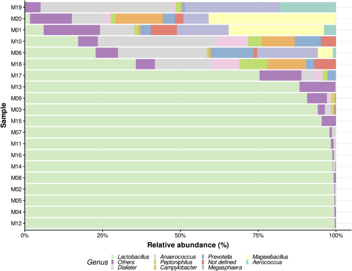
Bar plot of the top ten most abundant genera across all analyzed vaginal 16S samples. The bars represent relative abundances estimated by Emu for each sequenced sample, displaying only the top ten genera. Remaining genera are grouped as “Others.” The x-axis indicates the percentage of estimated abundances, while the y-axis lists samples ordered ascendingly by Lactobacillus abundance. The “Not defined” category corresponds to a particular taxon (Peptostreptococcaceae bacterium oral taxon 929) that lacks an assigned genus in the database used for analysis.
The second most abundant classification was the “Others” category, encompassing less represented genera that did not rank among the top 10. This pattern suggests that in samples dominated by Lactobacillus, the less abundant genera are a mix of low-abundance taxa without a consistent secondary dominant genus. Conversely, in the six samples where Lactobacillus relative abundance fell below 50%, the second most abundant, and in some cases, the dominant genus was Dialister. This genus and others evenly represented in these samples align with CST IV composition, characterized by the absence of a dominant genus44.
Relative abundances were analyzed at the species level, with results presented in Fig. 3, while the complete dataset is available in Supplementary Table S5. Among the Lactobacillus species, L. crispatus, L. iners, and L. gaseri were the most relatively abundant, correlating strongly CST I, II, and III, respectively23. These species exhibited relative abundances often exceeding 90% in dominant samples, such as M07, M12, and M14. Notably, 7 out of the 20 samples exhibited a relative abundance of L. crispatus above 80%, aligning with healthy vaginal microbiota profiles. Interestingly, only one sample (M11) showed a dominant abundance of L. jensenii (98%), which is characteristic of CST V. It is also noteworthy that in cases where L. iners was the most abundant species (M05, M09, M13), its relative abundance never exceeded 80%, and the second most abundant species was also a Lactobacillus species.
Fig. 3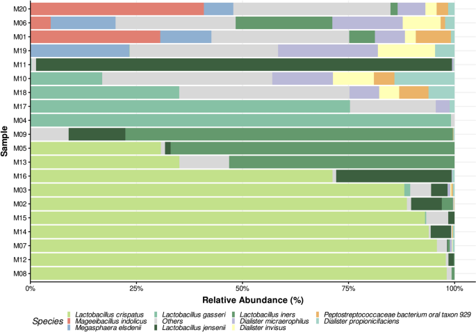
Bar plot of the top ten most abundant species across all analyzed vaginal 16S samples. The bars represent the species relative abundances estimated by Emu for each sequenced sample, displaying only the top ten most abundant across all samples. Remaining species are grouped as “Others.” The x-axis indicates the percentage of estimated abundances, while the y-axis lists samples ordered ascendingly by species from the Lactobacillus genus abundance.
Samples with reduced Lactobacillus dominance, such as M01 and M19, displayed more diverse microbial communities, including significant proportions of Mageeibacillus indolicus (30.6% in M01) and Megasphaera elsdenii (23.2% in M19). The “Others” category, representing less abundant taxa, contributed up to 30–40% in the more diverse samples (M01, M06, M10, M18, M19, M20), indicating substantial microbial complexity. Samples M19 and M20, where Lactobacillus species were minimal, exhibited a marked increase in diversity, with dominance by genera such as Mageeibacillus and Megasphaera. This shift toward increased diversity and reduced Lactobacillus dominance is consistent with CST IV profiles.
Considering that the species-level analysis yielded results consistent with previously reported key taxa and relative abundances characteristic of each CST, we performed a preliminary classification of the samples into groups based on these features. Samples were classified according to their dominant species, defined as the species representing more than 80% of the total relative abundance. The results of this preliminary classification are presented in Table 6.
Table 6 Classification of samples into groups based on relative abundances of Lactobacillus species.Diversity analysis of vaginal microbiome samplesGenus diversity analysis correlates with a potential dysbiosis state
We conducted a diversity analysis at the genus level to evaluate the information provided at this taxonomic resolution and compare it with species-level resolution. This comparison aims to highlight the advantages of full-length 16S rRNA gene sequencing. Alpha diversity, measured using the Shannon and Simpson indices, was calculated for each sample at the genus level. The results are presented in Supplementary Fig. 2, with statistical comparisons of the diversity indices across previously determined groups shown in Supplementary Table S6. As expected, samples classified in group IV exhibited the highest diversity among all groups. Although the sample size is limited, group I had the lowest mean diversity, suggesting that Lactobacillus predominantly dominates this state with minimal presence of other bacterial genera. Given that group IV is consistent with CST IV, which is often associated with a potential dysbiotic state, its significantly higher mean diversity suggests that alpha diversity at the genus level may serve as an indicator of dysbiosis when considered independently.
A similar analysis was performed for beta diversity at the genus level using Bray–Curtis distance, with results shown in Supplementary Fig. 3. Principal component analysis results are provided in Supplementary Tables S7 and S8. Similar to the alpha diversity analysis, all samples clustered according to their previously determined groups. These results indicate that, at the genus level, it is not possible to distinguish between the different Lactobacillus-dominated groups. Still, samples corresponding to the diverse group IV can be separated. In Fig. 5, the principal component on the X-axis explains 75.2% of the variance, demonstrating that this type of analysis at the genus level provides a strong statistical representation. The loading analysis further indicates that the primary contributors to this separation are the relative abundances of Lactobacillus and various other bacterial genera.
Species-level diversity analysis allows community state classification
To further assess taxonomic resolution and validate the CST classification of our samples, we first conducted a beta diversity analysis at the species level using Bray–Curtis distance (Fig. 4). Additional results are provided in Supplementary Tables S9 and S10. The results show that samples clustered according to the preliminary groups and their correlative Community State Types (CSTs), supporting the classification based on dominant species and confirming concordance with previously defined CST structures. Statistical grouping analysis showed that the PERMANOVA test was significant (p = 0.001, R2 = 0.79), indicating strong differences among CSTs. However, PERMDISP was also significant (p = 0.001), suggesting that part of the observed separation may be attributed to differences in group dispersion, an effect likely amplified by the relatively small number of samples per CST. To complement these findings, we also analyzed alpha diversity grouped by CSTs (Fig. 5; Supplementary Table S11). CST IV exhibited the highest diversity values, with an average Shannon index of 2.42 and Simpson index of 0.851, indicating a more heterogeneous bacterial composition. In contrast, CSTs dominated by Lactobacillus species (I, II, III, and V) displayed lower diversity values, consistent with a more uniform microbiota. These results support the use of alpha diversity as a quantitative marker of potentially dysbiotic states and further highlight the added value of species-level analysis in distinguishing CSTs. Unlike the genus-level analysis, species-level beta diversity enabled a clearer separation between all CSTs, reflecting a finer resolution of microbial composition. The first principal component (X-axis) explained 44% of the variance, indicating a more complex diversity distribution at the species level. Notably, CST IV showed the greatest dispersion, consistent with its highly diverse and heterogeneous microbial profile. This variability suggests possible sub-classifications within CST IV, potentially representing distinct dysbiotic states or ecological shifts. The loading analysis (highlighting the 15 most influential taxa) revealed that several species, including Neisseria gonorrhoeae, Prevotella corporis, and Campylobacter hominis, contribute significantly to CST IV differentiation, contrasting with taxa predominant in Lactobacillus-dominated CSTs.
Fig. 4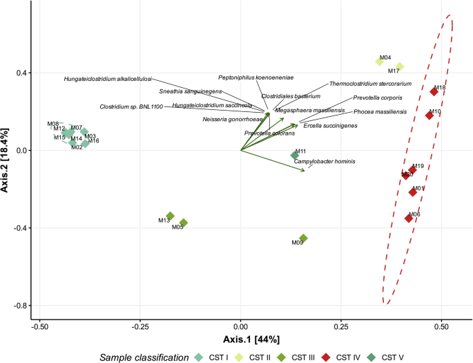
Beta diversity analysis by PCoA based on Bray–Curtis distance at the species level. The graph represents the Bray–Curtis distances of vaginal samples analyzed at the species level. Each sample is color-coded according to its previously determined community state (CST). Ellipses were added to group samples by CST; however, due to limited sample size, only CST I and CST VI are displayed. Principal Component Analysis (PCA) loadings are represented as arrows labeled with the corresponding species, showing only the 15 most contributing taxa. The x-axis represents the first principal component, while the y-axis represents the second principal component.
Fig. 5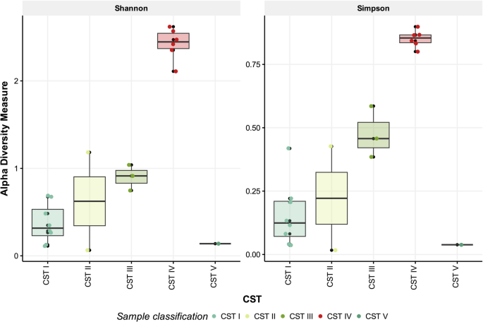
Alpha diversity analysis at the species level in vaginal samples. Boxplots represent species-level diversity in vaginal samples, grouped according to community state types (CSTs). CSTs include: CST I (L. crispatus-dominant), CST II (L. gasseri-dominant), CST III (L. iners-dominant), CST IV (high bacterial diversity), and CST V (L. jensenii-dominant). The x-axis displays the different CSTs, where each point represents an individual sample. The y-axis indicates alpha diversity, measured using Shannon and Simpson indices.