Photonic local oscillator
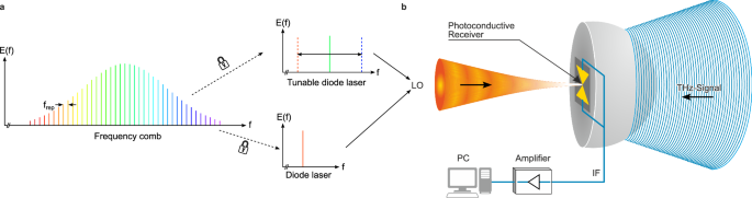
The laser engine, used as the LO, combines the stability and accuracy of comb technology with widely tunable CW external cavity diode-lasers (ECDL). The ECDL is optically phase-locked to a mode-locked erbium fiber laser comb with a fixed offset. For continuous phase-lock and tuning, the frequency comb is shifted with an external frequency shifter32 based on serrodyne shifting with 2π phase wrapping with an electro-optic phase modulator. The tunable CW ECDL follows the applied frequency shift of the optical comb while inheriting the stability of the comb within the locking bandwidth. The CW laser covers a mode-hop free tuning wavelength range of 100 nm ( > 12 THz) around 1550 nm within its and the comb’s spectrum. The external frequency shifting simultaneously minimizes spurious signals in the vicinity of the relevant mode. Pairing the tunable CW laser with a fixed CW laser enables the generation of THz difference frequencies. In this case the phase noise of the difference frequency signal is given by the quadratically scaling phase noise of the optical comb with frequency34 and the additive noise of the CW lasers. Additionally, combining the CW signals with a short pulse output of the frequency comb enables hybrid time- and frequency-domain measurements. Within the system all outputs are locked to the FC. Stabilizing the comb spectrum defines the noise properties. The comb has the option to absolutely reference it to a reference oscillator, e.g., an OCXO, which itself can be disciplined, e.g., to GPS, for SI traceable measurements. The referencing happens with a control circuit that matches the 4th harmonic of the repetition rate of the FC (200 MHz) to the frequency of the OCXO (800 MHz).
Photonic mixer
The photonic mixer driven by the comb-referenced LO is a photoconductor optimized for operation at THz frequencies. Details on the used material Rh:InGaAs as well as typical antenna and electrode designs, can be found elsewhere10,29,30. In the following we only describe the working principle of the photoconductive continuous-wave LO in general. The two tones generated by the LO result in a beat note with a time-dependent laser power of
$${P}_{L}\left(t\right)={P}_{L,0}(1+\cos [\left({\omega }_{1}-{\omega }_{2}\right)t+{\varphi }_{1}-{\varphi }_{2}])={P}_{L,0}(1+\cos \left[2\pi {f}_{{LO}}t+{\varphi }_{{LO}}\right])$$
(1)
where we define the local oscillator frequency as the frequency difference of the two tones,\(\,{f}_{{LO}}=\left|{\omega }_{1}-{\omega }_{2}\right|/2\pi\). \({\varphi }_{1}\) and \({\varphi }_{2}\) are the phases of the optical carrier waves and \({\varphi }_{{LO}}={\varphi }_{1}-{\varphi }_{2}\) is the resulting envelope phase. The photoconductor absorbs the beat note generated by the LO, resulting in a conductivity modulation of \(\sigma \sim {P}_{L}(t)\), by generating electron-hole pairs. The proportionality factor depends on a series of parameters, such as the absorption coefficient of the photoconductive layer stack but also the carrier lifetime and mobility of the material and the electrode geometry. The antenna attached to the photoconductor receives at the same time the electric field \({E}_{{SUT}}\left(t\right)\) emitted by the source under test (SUT) and converts it to a voltage, resulting in a net current of
$${I}_{{IF}}\left(t\right) \sim {P}_{L}\left(t\right){E}_{{SUT}}\left(t\right)$$
(2)
The proportionality factor depends again on a variety of parameters, such as the antenna’s radiation resistance, the RC roll-off caused by the combination of the antenna with the photoconductor’s capacitance and a lifetime roll off. Generally speaking, the prefactor decreases with increasing frequency beyond a few 100 GHz.
For a delta-shaped, spectrally pure LO as approximately provided by the comb-referenced LO and a single frequency SUT with an electric field of \({E}_{{SUT}}\left(t\right)={E}_{{SUT},0}\cos (2\pi {f}_{{SUT}}t+{\varphi }_{{SUT}})\), the IF current (i.e. the frequency component closest to DC; THz components are ignored as they are filtered out by slow post detection electronics) becomes
$${I}_{{IF}}\left(t\right) \sim {P}_{L,0}{E}_{{SUT},0}\cos \left[2\pi \left({f}_{{LO}}-{f}_{{SUT}}\right)t+{\varphi }_{{LO}}-{\varphi }_{{SUT}}\right]$$
(3)
If SUT and LO are not phase-locked as in case of the spectrum analyzer, the phase difference \({\varphi }_{{LO}}-{\varphi }_{{SUT}}\) fluctuates randomly over time. Thus, the time-averaged current in Eq. (3) is zero. However, its power spectral density, \({PS}{D}_{I}\) remains finite, also for energy conservation reasons,
$${PS}{D}_{I}\left(f,\,{f}_{{LO}}-{f}_{{SUT}}\right)={\left|{{\mathscr{F}}}\left\{I\left(t\right)\right\}\right|}^{2} \sim {P}_{L,0}^{2}{E}_{{SUT},0}^{2}\delta (f-{{|f}}_{{LO}}-{f}_{{SUT}}|)$$
(4)
where \({{f}_{{IF}}={|f}}_{{LO}}-{f}_{{SUT}}|\) is the intermediate frequency where the power spectral density appears and ℱ(.) is the Fourier transformation. If the SUT features a finite bandwidth the process will map the THz bandwidth to the IF domain. In practice, the IF current in Eq. (3) generated by the photoconductor is pre-amplified by a transimpedance amplifier (TEM Messtechnik PDA-S or Femto DHPCA-100) and subsequently digitized by an analog-to digital conversion card (Advantech PCIE-1840L). The PSA in this manuscript employs two detection methods to determine the PSD of the SUT22. The first requires the LO to be set to one frequency during the course of the measurement. During the measurement time, the time-domain signal is acquired, Fourier transformed and finally squared, providing a “snapshot” of the spectrum around the LO frequency. To cover a larger frequency range, multiple of these are put together using slightly different LO frequencies. The second employs a (digital) low-pass filter in the IF-domain. For this the LO frequency needs to be swept from a starting to an end frequency with a known speed. Any part of the signal that falls into the low-pass filter will be acquired. Finally, squaring the signal provides the PSD~\({E}_{{SUT},0}^{2}\) of the SUT. Alternatively, the PSD can be directly read out with a low frequency electronic spectrum analyzer operating in the IF domain40. The only missing step is a power calibration in order to determine the spectral power density of the received THz wave.
IF Tx and Rx are phase-locked, as in the case of the CW spectrometer operated with the same photonic LO, the phase difference in Eq. (3) does not average out. Further, for the homodyne case \({f}_{{LO}}-{f}_{{SUT}}=0.\) Thus, the IF current becomes time-independent, \({I}_{{IF}} \sim {P}_{L,0}{E}_{{SUT},0}\cos [{\varphi }_{{Tx}}-{\varphi }_{{Rx}}]\). Usually, there is a path length difference between the point where Tx laser signal and Rx laser signal are split and the position of the Rx. This optical path length difference \(\Delta ({{\rm{n}}}l)\) results in a linear frequency dependence of the phase difference, \({\varphi }_{{Tx}}-{\varphi }_{{Rx}}={k}_{0}\Delta \left({{\rm{n}}}l\right)=2\pi c\Delta \left({{\rm{n}}}l\right){f}_{{LO}}\sim {f}_{{LO}}\) oscillates with the THz frequency, causing homodyne fringes. Figure 7b plots the amplitude of the homodyne fringes vs. THz frequency.
Linewidth and spectral resolution
For simplicity, we assume for now Gaussian spectral shapes of the form
$$E\left(f\right)={E}_{0}\exp \left(-\frac{{(f-{f}_{L})}^{2}}{{\sigma }^{2}}\right)$$
(5)
where \(\sigma\) is the \({e}^{-2}\) width of the spectral power (\({e}^{-1}\) width of the field) and \({f}_{L}\) the (positive-valued) laser frequency. The envelope of the heterodyned optical wave originates from a product of the fields at the respective colors in the time domain. Spectrally, the product turns into a convolution. For two Gaussian shapes of widths \({\sigma }_{L1}\) and \({\sigma }_{L2}\) results in a Gaussian with a combined linewidth of the photonic LO of \({\sigma }_{{LO}}=\sqrt{{\sigma }_{L1}^{2}+{\sigma }_{L2}^{2}\,}\). Subsequently, the envelope with a spectral width of \({\sigma }_{L}\) is convoluted with the THz wave with a spectral width of \({\sigma }_{{THz}}\) leading to a combined linewidth of \({\sigma }_{{tot}}=\sqrt{{\sigma }_{{LO}}^{2}+{\sigma }_{{SUT}}^{2}\,}\). Therefore, with the knowledge of the linewidth of either the SUT or the LO, the respective other one can be calculated. In any case, both are smaller than the measured linewidth \({\sigma }_{{tot}}\). For Lorentzian or Voigt spectral profiles, it is qualitatively similar, though mathematically more complicated.
Power calibration
The power of the spectra is calibrated with the responsivity \({{\mathscr{R}}}\) of the Rh:InGaAs photoconductive receiver. The determination of the responsivity requires information on the resulting photocurrent \({I}_{{IF}}\) of a homodyne or heterodyne measurement setup with the photoconductive receiver and a measurement of the THz power \({P}_{{cal}}\) of the homodyne system. The responsivity is given as
$${{\mathscr{R}}}\left(f\right)=\frac{{I}_{{IF}}^{2}(f)}{{P}_{{cal}}(f)}$$
(6)
Generally speaking, reliable power detection in the THz domain is very challenging and afflicted by large errors. For the power calibrations, we used a pyroelectric detector, calibrated to Si-units at the German national metrology institute PTB (SLT Sensor- und Lasertechnik, THz10). Due to differences in the calibration frequency of 1.4 THz and the measured frequencies, we assume a maximum frequency-dependent error of 30%. The pyroelectric detector has a noise equivalent power of 1 µW which enabled the calibration of the photoconductive receiver for the frequency range between 50 GHz and 1.6 THz. For higher frequencies, the source power of the calibration source is below the detection limit of the pyroelectric detector. Therefore, we extrapolated the responsivity for higher frequencies taking into account lifetime and RC roll-off of the photoconductor above 1.1 THz. To confirm the responsivity values, we additionally investigated a CW THz source at a frequency of 95 GHz with the PSA and measured its source power.
Signal-to-noise ratio
The signal-to-noise ratio (SNR) within the measurements is dependent on the noise floor and responsivity of the receiver side, the THz power from the emitter and the linewidth of the signal-under-test and of the LO. All of the sources shown in this manuscript use photomixers (pin diodes or photoconductors) to generate the THz signal. Independent of the used optical signal (pulsed or CW), the power of the signal decreases with increasing frequency for frequencies higher than the roll-off 3dB-frequencies. For the pulsed variant, additionally, fewer optical modes mix with each other with increasing frequency, further reducing the signal power. The signal path consists in most cases of two parabolic mirrors in a U-configuration, Si lenses and InP substrate within the photomixer’s package and a free-space path of less than 0.5 m. Along the signal path losses, reflection and absorption (i.e., water vapor, see also Fig. 7b) may occur reducing the signal strength inbound to the receiver. The photocurrent generated by the receiver depends on the strength of the incoming electrical field (see Eq. (2)) and the LO frequency. Roll-off effects within the photomixer reduce its responsivity with increasing LO frequency. The noise current of the photomixer is mostly independent of the LO frequency. The lower responsivities at higher frequencies thus require larger signals for successful detection. Additionally, the noise floor is directly proportional to the measurement bandwidth. Smaller measurement bandwidths (i.e., longer integration times) allow for the detection of smaller signals. The system-specific noise floor is therefore frequently given in the unit dB/Hz.
The bandwidth is limited on the lower end by the LO linewidth. The system essentially measures the spectral density, i.e., the power of the signal within a measurement bandwidth (frequency bin). Spectrally wide LOs or signals -such as the one in Fig. 2 are distributed over many frequency bins, reducing the power per bin and thus the signal to noise ratio. As the responsivity of the photoconductors drops with increasing frequency, smaller SNRs lead to smaller usable bandwidths, ranging from DC to the maximum still detectable signal. The result is a lower achievable measurement bandwidth in case of a non-referenced CW signal, while the usable measurement bandwidth increases with better relative stability between the SUT and LO enabling a measurement bandwidth of 6.5 THz with all spectral power concentrated within a 2 Hz frequency bin.
Pressure and temperature broadening
The lifetime of the rotational state \(\tau\) of a molecule limits its natural linewidth (typ. 10–100 s kHz) and features a Lorentzian spectral distribution \(p\left(f\right)\),
$$p\left(f\right)=\frac{A}{{\left(f-{f}_{0}\right)}^{2}+\left(\frac{1}{\pi \tau }\right)}$$
(7)
When two gas molecules collide or their dipole moments perturb each other during a pass by maneuver, the lifetime of the rotational state is lowered. The more molecules per volume are present (i.e. the higher the pressure) the shorter the respective lifetime and the larger the linewidth according to Eq. (7). The pressure broadened linewidth is directly proportional to the pressure, has a Lorentzian shape and reaches linewidths in the few GHz range at normal pressure50. We remark that heavier molecules have larger impact such that foreign gases will cause a different linewidth as a pure gas. In ambient conditions the absorption also experiences Doppler broadening caused by thermal motion of the gas molecules towards and away from the THz source. The Doppler broadening \({\varDelta f}_{D}\) is given by ref. 51
$${\varDelta f}_{D}=f\sqrt{\frac{8{\mathrm{ln}}\left(2\right){k}_{B}T}{m{c}^{2}}}$$
(8)
where \(f\) is the center frequency, \({k}_{B}\) the Boltzmann constant, \(T\) the temperature and \(m\) the molecule’s mass. Based on statistical motion of the molecules, Doppler broadening features a Gaussian line shape. The theoretical Doppler limit for water vapor is 1.62 MHz at the 556.936 GHz line at a room temperature of 23 °C.
For the measurements with water vapor under vacuum, we used a spectroscopy setup with a vacuum tube in the THz beam. Beamforming equipment in the form of two lenses and photoconductive transmitter and receiver were outside the vacuum tube, purged with dry air to prevent water absorption at normal pressure outside the tube. A combined membrane pump with a turbomolecular pump enabled pressures as low as 0.001 mbar within the tube. Additional water in form of an ammonia-water solution is added in an extended part of the tube that is separated by a needle valve. For the measurements the needle valve is opened slightly to let water vapor into the tube and depending on the pressure the pumps closed off of the tube. Each measurement consists of three runs of five seconds where each run contains one up and one down scan. During each measurement we monitored the pressure with a pressure gauge. The pressure within the tube changed on average by a factor of 1.5 as the tube is quite leaky. Therefore, each measurement is compared to the maximum pressure within its measurement time window. The pressure gauge has an error of 20% due to a lack of recent calibration. The tube does not contain heating or cooling equipment and was left at room temperature (23 °C), limiting the measurements to the Doppler broadened spectra. The absorption coefficient\(\,\alpha\) is calculated by
$$\alpha=-\frac{{{\mathrm{ln}}}\left(\frac{{I}_{{H}_{2}O}}{{I}_{0}}\right)}{d}$$
(9)
where \({I}_{0}\) is the intensity of the reference measurement, \({I}_{{H}_{2}O}\) the water vapor measurement and \(d\) = 33 cm the mean THz path length inside the vacuum tube.