DatasetsVegetation cover data
The Vegetation Continuous Fields version 1 product (VCF5KYR) was adopted to provide global fine-scale fractional vegetation cover information14. This product has a 0.05° × 0.05° spatial resolution and a yearly interval, combining the advantages of multiple satellite sensors with very high spatial resolutions. The product is available from 1982 to 2016 and features the percentage of tree cover (tall vegetation ≥ 5 m in height, abbreviated as \({{\rm{TC}}}\)), short vegetation (\({{\rm{SV}}}\)), and bare ground (\({{\rm{BG}}}\)), respectively for land pixels, with a precision of 1%, representing the vegetation composition of each pixel during the peak growing season14. The sum of the proportions of the three land-cover types for each pixel is 100%. The spatial pattern of global vegetation cover and the dominant changes in vegetation cover type are shown in Supplementary Fig. 3. Note that the years 1994 and 2000 were excluded from analyses due to a lack of VCF5KYR data (https://lpdaac.usgs.gov/products/vcf5kyrv001/). The broad vegetation cover classification was adopted in order to maximize the utility of the available data while ensuring the statistical significance and robustness of the results. Despite the inherent resolution limitation, our approach provides valuable information on VCC at a scale that is consistent with the LAI data.
LAI data
Our analysis involved the examination of four LAI products covering the satellite era, including the Advanced Very High-Resolution Radiometer (AVHRR) Global Inventory Monitoring and Modeling Studies (GIMMS) LAI3g dataset3,49, the National Oceanic and Atmospheric Administration (NOAA) Climate Data Record (CDR)50, the Global Land Surface Satellite (GLASS) AVHRR LAI V50 product51, and the GLOBMAP LAI V3 (ref52.), all of which aim to provide consistent and reliable attributions of global LAI change. Note that while LAI serves as a valuable proxy of vegetation greenness11,53, it may be subject to saturation effects in areas with dense vegetation, similar to other vegetation indices54,55. In addition, estimating LAI from satellite imagery comes with several well-known limitations2,56,57,58,59. These include spatial resolution constraints, saturation in densely vegetated areas, orbital drift, sensor replacements, retrieval algorithm uncertainties, and disturbances from land-cover heterogeneity, cloud contamination, and background reflectance. Despite these challenges, our data-driven analysis offers critical insights into the impact of VCC on LAI, allowing us to uncover broad trends and patterns across large spatial scales.
Our findings are based on the AVHRR GIMMS LAI3g dataset3,49 (see Robustness Analysis), which provides a comprehensive and continuous time series of LAI during the period from 1982 to 2015. Generated based on a Feed-Forward Neural Network (FFNN) model, it has a spatial resolution of 1/12°, is a bi-monthly composite, and has global coverage. It is one of the longest series among current LAI datasets and has demonstrated good performance in representing vegetation dynamics3,10,11. We first interpolated the GIMMS LAI3g into 0.05° grid spacing by using linear interpolation to fit the VCF5KYR land-cover data and averaged LAI into a monthly scale by taking the temporal mean of all valid records. We then retrieved the maximum monthly LAI that represents the peak vegetation growth35 for each pixel in each year. We calculated the annual mean LAI simultaneously to discuss the uncertainties associated with the proxy of vegetation greenness (Supplementary Fig. 10; Robustness Analysis). The quantitative attributions of long-term LAI changes were determined for the period from 1982 to 2015 to align with the availability of VCF5KYR and LAI products.
To provide a robust assessment associated with satellite-based products, we utilized LAI data from three alternative long-term satellite products to examine attributions of LAI change: NOAA CDR50, which spans from July 1981 to the present with daily frequency and a 0.05° resolution (Supplementary Fig. 11); GLASS51, which offers 8-day LAI data with a spatial resolution of 0.05° and covers the period from 1981 to 2018 (Supplementary Fig. 12); GLOBMAP52, which offers biweekly LAI data during 1981–2000 and 8-day LAI data during 2001–2020 at 8 km resolution (Supplementary Fig. 13). All LAI datasets were interpolated to a 0.05° grid spacing and aggregated into monthly scales for analyses.
Disentanglement of the vegetation greenness
As shown in Supplementary Fig. 1, the main concept of our framework contains two parts. Developing such a framework is motivated by the lack of LAI observations for specific vegetation types, as existing LAI data are grid-based at a resolution of ~ 5 kilometers, with each grid cell representing a single value that averages across multiple vegetation types. This means the lack of information on individual vegetation types for LAI, making it difficult to quantify how sub-grid scale vegetation cover changes contribute to overall LAI variations.
The first step is elucidating the proportion of different vegetation cover types from satellite-observed LAI based on an improved Bounded-Variable Least Squares (BVLS) model60 (Eqs. 1–3). In our study, we extended the traditional BVLS approach by not only defining value ranges for the three greenness variables (\({{{\rm{\beta }}}}_{{{\rm{TC}}}}\), \({{{\rm{\beta }}}}_{{{\rm{SV}}}}\), \({{{\rm{\beta }}}}_{{{\rm{BG}}}}\)) but also imposing additional constraints on their relative magnitudes (Eq. 3 and Supplementary Fig. 19). These improvements ensured that the estimated parameters adhered to physically meaningful relationships, enhancing the stability and reliability of the results, especially under conditions of noise or multicollinearity. High-resolution satellite-observed LAI data (e.g., Supplementary Fig. 2) and the VCF5KYR product14 (Supplementary Fig. 3) during 1982–2015 are used as inputs for the statistical model. To overcome the spatial homogeneity issue raised by the coarse precision of VCF data, the percentage of TC, SV, and BG, as well as the LAI data, all at 0.05° × 0.05° resolution, were first aggregated to 0.1° × 0.1° cells for each year by taking the average of all valid records. These 0.1° cells were then used as input to the BVLS regression. We used 3° × 3° grid spacing as the analysis unit and retained only the grids and their inside cells with more than 20% valid LAI and vegetation cover observations at their original resolution. For detailed discussion regarding the size of cells and grids, please refer to Robustness Analysis.
We decomposed the observed LAI to TC, SV, and BG at the 3° × 3° grid level for each year (Supplementary Fig. 1). The following regression was established for each valid 0.1° × 0.1° cell to account for the quantitative relationship between LAI and vegetation cover in the current 3° × 3° grid:
$$\left\{\begin{array}{c}{{{\rm{LAI}}}}_{1}={{{\rm{\beta }}}}_{{{\rm{TC}}}}\cdot {{{\rm{TC}}}}_{1}+{{{\rm{\beta }}}}_{{{\rm{SV}}}}\cdot {{{\rm{SV}}}}_{1}+{{{\rm{\beta }}}}_{{{\rm{BG}}}}\cdot {{{\rm{BG}}}}_{1}+{{{\rm{\varepsilon }}}}_{1}\\ {{{\rm{LAI}}}}_{2}={{{\rm{\beta }}}}_{{{\rm{TC}}}}\cdot {{{\rm{TC}}}}_{2}+{{{\rm{\beta }}}}_{{{\rm{SV}}}}\cdot {{{\rm{SV}}}}_{2}+{{{\rm{\beta }}}}_{{{\rm{BG}}}}\cdot {{{\rm{BG}}}}_{2}+{{{\rm{\varepsilon }}}}_{2}\\ \ldots \\ {{{\rm{LAI}}}}_{{{\rm{i}}}}={{{\rm{\beta }}}}_{{{\rm{TC}}}}\cdot {{{\rm{TC}}}}_{{{\rm{i}}}}+{{{\rm{\beta }}}}_{{{\rm{SV}}}}\cdot {{{\rm{SV}}}}_{{{\rm{i}}}}+{{{\rm{\beta }}}}_{{{\rm{BG}}}}\cdot {{{\rm{BG}}}}_{{{\rm{i}}}}+{{{\rm{\varepsilon }}}}_{{{\rm{i}}}}\\ \ldots \\ {{{\rm{LAI}}}}_{{{\rm{n}}}}={{{\rm{\beta }}}}_{{{\rm{TC}}}}\cdot {{{\rm{TC}}}}_{{{\rm{n}}}}+{{{\rm{\beta }}}}_{{{\rm{SV}}}}\cdot {{{\rm{SV}}}}_{{{\rm{n}}}}+{{{\rm{\beta }}}}_{{{\rm{BG}}}}\cdot {{{\rm{BG}}}}_{{{\rm{n}}}}+{{{\rm{\varepsilon }}}}_{{{\rm{n}}}}\end{array}\right.$$
(1)
where \({{\rm{n}}}\) is the number of valid cells with a maximum of 900; \({{{\rm{LAI}}}}_{{{\rm{i}}}}\) is the satellite-observed LAI value at cell \({{\rm{i}}}\); \({{{\rm{TC}}}}_{{{\rm{i}}}}\), \({{{\rm{SV}}}}_{{{\rm{i}}}}\), and \({{{\rm{BG}}}}_{{{\rm{i}}}}\) are the percentage of TC, SV, and BG at cell \({{\rm{i}}}\), respectively, and their sum equals 100%; \({{{\rm{\beta }}}}_{{{\rm{TC}}}}\), \({{{\rm{\beta }}}}_{{{\rm{SV}}}}\), and \({{{\rm{\beta }}}}_{{{\rm{BG}}}}\) represent the estimated LAI parameter (in m2 m−2) of the current 3° × 3° grid for assumed 100% coverage of TC, SV, and BG, respectively. Our improved BVLS model solves the linear least-squares regression with upper and lower bounds on the parameters (i.e., \({{{\rm{\beta }}}}_{{{\rm{TC}}}}\), \({{{\rm{\beta }}}}_{{{\rm{SV}}}}\), and \({{{\rm{\beta }}}}_{{{\rm{BG}}}}\)), given as:
$${\min }_{{{\rm{l}}}\le {{\rm{x}}}\le {{\rm{u}}}}{{\rm{||Ax}}}-{{\rm{b}}}{||}_2$$
(2)
where \({{\rm{A}}}\) is an \({{\rm{n}}}\)-by-3 matrix of observed vegetation cover, \({{\rm{b}}}\) is an \({{\rm{n}}}\)-by-1 vector of observed LAI. Specifically, the parameters are constrained by the following inequality with upper and lower (non-negative) limits:
\({{{\rm{\beta }}}}_{\max }\) was defined individually for each grid in each year based on the observation. This inequality was verified using a stratified random-sample approach (details refer to Supplementary Fig. 19). The significance of F-statistics (p-value) and the coefficient of determination (R2) for the BVLS model were calculated to show the goodness of fit in estimating vegetation greenness parameters. The F-test, with a significance level of p-value 2 reflects how well the model explains the pixel-level (0.1°) LAI variation using the grid-level averaged greenness parameters (\({{\rm{\beta }}}\)) within a 3° × 3° grid. Note that the R2 value could be negative, indicating that the improved BVLS model with constraints is not appropriate for the samples.
The improved BVLS model was established and solved in each 3° × 3° grid for each year. The models with low confidence were removed based on the model parameters (i.e., a p-value of F-statistics > 0.05 and/or negative R2). Grids were retained only if they had at least 16 years of credible BVLS models during the study period. Overall, there are 1544 valid grids left after the model quality assessment, accounting for 96.0% of all grids. Among them, 1299 grids (80.8%) have valid results in all 32 years (the years 1994 and 2000 were excluded from analyses due to a lack of VCF data). The model performs better (i.e., exhibits higher R2 values) in regions with LAI increase hotspots and/or significant vegetation cover change (e.g., East Asia, South Asia, Europe, Sahel, eastern South America, eastern Australia), while it shows lower R2 in areas with dense, uniform vegetation (e.g., the Amazon and Congo forests, and high-latitude tundra), likely due to limited variability in vegetation composition (Supplementary Fig. 4). The invalid grids are mainly located in coastal areas and tropical rainforests (Supplementary Fig. 4). Based on the improved BVLS statistical model and the high-resolution satellite-observed LAI and VCF data, we successfully disentangled the \({{{\rm{\beta }}}}_{{{\rm{TC}}}}\), \({{{\rm{\beta }}}}_{{{\rm{SV}}}}\), and \({{{\rm{\beta }}}}_{{{\rm{BG}}}}\) parameters for each 3° × 3° grid and each year (Supplementary Fig. 5).
Attribution of Earth’s LAI response to vegetation cover change
In the second step of our framework, we reconstructed annual LAI values by using the parameters retrieved from the BVLS model. For each 3° × 3° grid in each year, the LAI value (\({{\rm{\sigma }}}{{\rm{LAI}}}\); in m2 m−2) was calculated as:
$${{\rm{\sigma }}}{{\rm{LAI}}}={{{\rm{\beta }}}}_{{{\rm{TC}}}}\cdot {{\rm{TC}}}+{{{\rm{\beta }}}}_{{{\rm{SV}}}}\cdot {{\rm{SV}}}+{{{\rm{\beta }}}}_{{{\rm{BG}}}}\cdot {{\rm{BG}}}$$
(4)
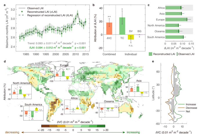
where \({{\rm{TC}}}\), \({{\rm{SV}}}\), and \({{\rm{BG}}}\) are the mean proportion (%) of tree cover, short vegetation, and bare ground averaged from the valid cells in the current grid. For regional and global analyses, the grid-level estimations of LAI were aggregated by taking the area-weighted average approach, with the upper and lower ranges of the 95% confidence interval being estimated. The long-term trends of reconstructed LAI (refer to as \({{\rm{\delta }}}{{\rm{LAI}}}\)) were derived by using linear regression during the study period at the grid, regional and global scales. The upper and lower ranges of \({{\rm{\delta }}}{{\rm{LAI}}}\) were estimated based on the standard error of the mean. Generally, the reconstructed \({{\rm{\delta }}}{{\rm{LAI}}}\) performs very well in reproducing the trend and variation of the observed LAI dynamics across the global, continental, and regional scales (details refer to Validation).
To attribute the reconstructed LAI trends to drivers related to VCC, we differentiated Eq. (4) with respect to the year (denoted as \({{\rm{y}}}\)), as follows:
$${{\rm{\delta }}}{{\rm{LAI}}}= \frac{\partial {{\rm{\sigma }}}{{\rm{LAI}}}}{\partial {{\rm{y}}}}=\frac{\partial {{{\rm{\beta }}}}_{{{\rm{TC}}}}}{\partial {{\rm{y}}}}\cdot \overline{{{\rm{TC}}}}+\frac{\partial {{\rm{TC}}}}{\partial {{\rm{y}}}}\cdot \overline{{{{\rm{\beta }}}}_{{{\rm{TC}}}}}+\frac{\partial {{{\rm{\beta }}}}_{{{\rm{SV}}}}}{\partial {{\rm{y}}}}\cdot \overline{{{\rm{SV}}}} \\ + \frac{\partial {{\rm{SV}}}}{\partial {{\rm{y}}}}\cdot \overline{{{{\rm{\beta }}}}_{{{\rm{SV}}}}}+\frac{\partial {{{\rm{\beta }}}}_{{{\rm{BG}}}}}{\partial {{\rm{y}}}}\cdot \overline{{{\rm{BG}}}}+\frac{\partial {{\rm{BG}}}}{\partial {{\rm{y}}}}\cdot \overline{{{{\rm{\beta }}}}_{{{\rm{BG}}}}}$$
(5)
where the overbar denotes the multi-year average value of the variable. On the right-hand side of Eq. (5), the six terms represent the changes in reconstructed LAI associated with the changes in the greenness of tree cover (\({{{\rm{\beta }}}}_{{{\rm{TC}}}}\)), the proportion of tree cover (\({{\rm{TC}}}\)), the greenness of short vegetation (\({{{\rm{\beta }}}}_{{{\rm{SV}}}}\)), the proportion of short vegetation (\({{\rm{SV}}}\)), the greenness of bare ground (\({{{\rm{\beta }}}}_{{{\rm{BG}}}}\)) and the proportion of bare ground (\({{\rm{BG}}}\)), respectively.
The reconstructed \({{\rm{\delta }}}{{\rm{LAI}}}\) was further attributed to vegetation cover change (\({{\rm{\delta }}}{{\rm{VC}}}\)), given by:
$${{\rm{\delta }}}{{\rm{VC}}}=\frac{\partial {{\rm{TC}}}}{\partial {{\rm{y}}}}\cdot \overline{{{{\rm{\beta }}}}_{{{\rm{TC}}}}}+\frac{\partial {{\rm{SV}}}}{\partial {{\rm{y}}}}\cdot \overline{{{{\rm{\beta }}}}_{{{\rm{SV}}}}}+\frac{\partial {{\rm{BG}}}}{\partial {{\rm{y}}}}\cdot \overline{{{{\rm{\beta }}}}_{{{\rm{BG}}}}}$$
(6)
and the contributions of VCC were calculated as the ratio of \({{\rm{\delta }}}{{\rm{VC}}}\) to \({{\rm{\delta }}}{{\rm{LAI}}}\). Similarly, the attributions of the changes in the proportion of tree cover (\(\frac{\partial {{\rm{TC}}}}{\partial {{\rm{y}}}}\cdot \overline{{{{\rm{\beta }}}}_{{{\rm{TC}}}}}\)), short vegetation (\(\frac{\partial {{\rm{SV}}}}{\partial {{\rm{y}}}}\cdot \overline{{{{\rm{\beta }}}}_{{{\rm{SV}}}}}\)) and bare ground (\(\frac{\partial {{\rm{BG}}}}{\partial {{\rm{y}}}}\cdot \overline{{{{\rm{\beta }}}}_{{{\rm{BG}}}}}\)) were calculated at regional and global scales. The remaining part (\({{\rm{\delta }}}{{\rm{ID}}}\)) represents the LAI changes in constant vegetation, which is largely influenced by indirect factors, as given by:
$${{\rm{\delta }}}{{\rm{ID}}}=\frac{\partial {{{\rm{\beta }}}}_{{{\rm{TC}}}}}{\partial {{\rm{y}}}}\cdot \overline{{{\rm{TC}}}}+\frac{\partial {{{\rm{\beta }}}}_{{{\rm{SV}}}}}{\partial {{\rm{y}}}}\cdot \overline{{{\rm{SV}}}}+\frac{\partial {{{\rm{\beta }}}}_{{{\rm{BG}}}}}{\partial {{\rm{y}}}}\cdot \overline{{{\rm{BG}}}}$$
(7)
The interannual variations of the VCC-induced LAI (\({{{\rm{\sigma }}}{{\rm{VC}}}}_{{{\rm{y}}}}\); in m2 m−2) could be reconstructed using a variable-controlling approach61 by fixing the greenness of tree cover, short vegetation and bare ground as multi-year average values:
$${{{\rm{\sigma }}}{{\rm{VC}}}}_{{{\rm{y}}}}=\overline{{{{\rm{\beta }}}}_{{{\rm{TC}}}}}\cdot {{{\rm{TC}}}}_{{{\rm{y}}}}+\overline{{{{\rm{\beta }}}}_{{{\rm{SV}}}}}\cdot {{{\rm{SV}}}}_{{{\rm{y}}}}+\overline{{{{\rm{\beta }}}}_{{{\rm{BG}}}}}\cdot {{{\rm{BG}}}}_{{{\rm{y}}}}$$
(8)
The anomalies of \({{\rm{\sigma }}}{{\rm{VC}}}\) during the study period (e.g., Fig. 3a) were then obtained by subtracting the multi-year mean from the resulting time series. The variable-controlling approach was also applied spatially to calculate the contribution of LAI change within specific continents, countries, or regions to global \({{\rm{\delta }}}{{\rm{LAI}}}\) (Fig. 2c and Supplementary Table 2).
Estimating potential effect of stable cropland and managed forest
The global map of cropland extent62 spanning from 2003 to 2019, with a spatial resolution of 0.00025°, was utilized to delineate the extent of stable cropland without VCC signals. The original data were aggregated into 3° grid spacing using the area-weighted average approach, generating a global map showing the proportion of stable cropland (Supplementary Fig. 18a). Assuming that the LAI change of these areas is solely driven by human land-use practices, we estimated the potential contribution of cropland management (\({{\rm{\delta }}}{{\rm{SC}}}=\frac{\partial {{{\rm{\beta }}}}_{{{\rm{SV}}}}}{\partial {{\rm{y}}}}\cdot {{\rm{SC}}}\)) globally and regionally, where \({{\rm{SC}}}\) represents the proportion of stable cropland at the grid level. Note that this assumption may lead to an overestimation of the contribution by disregarding the background LAI change from indirect factors like CO2 fertilization, climate change and nitrogen deposition.
Validation
Our statistical models were validated for their ability to reproduce the characteristics of \({{\rm{\sigma }}}{{\rm{LAI}}}\) and \({{\rm{\delta }}}{{\rm{LAI}}}\) through comparisons with satellite-derived observations. At the grid level, the reconstructed annual \({{\rm{\sigma }}}{{\rm{LAI}}}\) shows high correlation coefficients (r > 0.99 for over 95.5% of valid 3° × 3° grids; Supplementary Fig. 6a) and minimal bias (2 m−2 for over 95.3% of grids; Supplementary Fig. 6b). Only slight overestimations occur in semi-arid regions, such as Central Asia and Sahel, while minor underestimations are mainly observed in tropical areas. For the reconstructed \({{\rm{\delta }}}{{\rm{LAI}}}\), more than 90% of the grids exhibit a bias of less than ± 0.01 m2 m−2 decade−1, with particularly low bias in grids with significant LAI changes (Supplementary Fig. 7). These results indicate that while the pixel-level fit of BVLS model may be moderate (R2 value of ~ 0.5 in Supplementary Fig. 4), our framework still captures grid-level signals effectively in terms of magnitude and interannual variability, as evidenced by high correlation coefficients and low bias metrics. Note that our attribution analysis focus on LAI dynamics at the 3° × 3° grid-level, and applying the estimated grid-average \({{\rm{\beta }}}\) values to disentangle and attribute LAI at finer scales (e.g., 0.1° × 0.1° pixels) may introduce uncertainty.
Overall, the results show high-quality performance globally with a high correlation coefficient (r = 0.997, p 1a and Supplementary Table 1) between the reconstructed annual LAI and the observations. On a continental scale, our reconstruction is robust in capturing the temporal variation and trend of the observed LAI, with correlation coefficient values varying from 0.977 to 0.999; and relative bias ranged between − 0.9% and 6.7% (Fig. 1c and Supplementary Table 1). In evaluating the model performance of the largest countries and regions, we show that our model had strong capability across most countries/regions, with correlation coefficient values larger than 0.97 and relative biases of less than 6% (Supplementary Table 1). The model is relatively weak in reproducing the trend of observed LAI change in Argentina and the Democratic Republic of the Congo. This difficulty likely stems from the low coefficient of determination for the BVLS model that was induced by the spatial homogeneity of vegetation cover in those grids.
The robustness analyses further confirmed the quality of our statistical models by demonstrating similar results when using the annual mean LAI (r = 0.990, p 10), the NOAA CDR LAI product (r= 0.993, p 11), the GLASS LAI product (r = 0.968, p 12), and the GLOBMAP LAI product (r = 0.990, p 13). For the three alternative LAI products, the reconstructed \({{\rm{\delta }}}{{\rm{LAI}}}\) also exhibits a low bias of less than ± 0.01 m2 m−2 decade−1 in 94.9%, 94.4%, and 81.6% of the grids, with particularly low bias in grids exhibiting significant LAI changes (Supplementary Fig. 20).
Robustness analysisGrid spacing
Initially, we conducted our analysis using a grid spacing of 0.5° × 0.5° as the analysis unit, with each grid containing up to 100 samples at the original 0.05° × 0.05° resolution. However, during the application of the improved BVLS models to those samples, we encountered approximately 40% of grids that produced models with low confidence, as indicated by a p-value of F-statistics > 0.05 and/or negative R2 (Supplementary Table 3). This can be attributed to the homogeneity of vegetation cover fraction caused by the relatively low precision (1%) of the VCF product14. At a local scale (i.e., 0.5° × 0.5° grid), many 0.05° × 0.05° cells shared the same fraction of tree cover and/or short vegetation due to the landscape similarities, yet exhibited different satellite-observed LAI values.
To tackle the issue of spatial homogeneity, we implemented a strategy involving spatial averaging of vegetation cover fractions and an increase in the number of samples at the grid level. We conducted experiments with various settings for grids and cells (Supplementary Table 3). Initially, the percentages of TC, SV, and BG, along with the LAI values at 0.05° × 0.05° resolution, were aggregated to cells ranging from 0.1° × 0.1° to 0.5° × 0.5° for each year. This involved calculating the average of all valid records within each cell. Subsequently, the BVLS models were established and solved at the grid level, with grid size ranging from 1° × 1° to 5° × 5°. Across different combinations of grid and cell sizes, the reconstructed contributions of \(\delta {VC}\) consistently ranged from 18.0% to 23.5%, underscoring the non-negligible role of VCC in global LAI increasing (Supplementary Table 3). Importantly, the robustness of our findings was not affected by the choice of analysis unit or spatial average window. Finally, we present the results based on a 3° × 3° grid spacing with a 0.1° × 0.1° spatial average window, which yielded the highest ratio of valid grids (96.0%) and a low bias (1.3%) in the reconstruction of \({{\rm{\delta }}}{{\rm{LAI}}}\).
Maximum monthly LAI and annual mean LAI
To assess the robustness of our proxy indicator of vegetation greenness, we investigated the uncertainties associated with different indices, comparing the results derived from annual mean LAI to those from maximum monthly LAI (Supplementary Fig. 8). The reconstructed global trend in annual mean LAI (0.030 ± 0.007 m2 m−2 decade−1; t(30) = 4.18, p p = 0.02) can be attributed to \({{\rm{\delta }}}{{\rm{VC}}}\), confirming the substantial impact of VCC. Furthermore, the spatial distribution of \({{\rm{\delta }}}{{\rm{VC}}}\) demonstrates a high level of consistency (Fig. 1 d versus Supplementary Fig. 8b). We report the results based on the maximum monthly LAI due to the following considerations: (1) it represents the peak vegetation greenness during the local peak growing season, a period identified by the vegetation fields data14; (2) it can better capture the interannual changes in the greenness of croplands and plantations with different cropping cycles, making it suitable for a global study35; (3) it is less affected by missing data and can be easily retrieved without subjectively defining a growing season or dealing with multiple growing seasons; and (4) the results have higher statistical significances compared with those derived from annual mean LAI.
LAI products
We performed the analysis using NOAA CDR50, GLASS51 and GLOBMAP52 as alternative products to the GIMMS LAI3g49 to test the uncertainties associated with different satellite-based datasets. Similarly, the reconstructed \({{\rm{\delta }}}{{\rm{LAI}}}\) based on these three datasets captures the observed magnitude and temporal variation of global vegetation greenness satisfactorily (Supplementary Figs. 11–13). Our findings consistently indicate that \({{\rm{\delta }}}{{\rm{VC}}}\) accounts for 14.6 ± 5.5% (t(30) = 2.88, p = 0.007), 34.5 ± 10.4% (t(30) = 3.30, p = 0.003) and 28.6 ± 11.8% (t(30) = 2.44, p = 0.021) of \(\delta {LAI}\) based on the NOAA CDR, the GLASS and the GLOBMAP products, respectively, reaffirming the validity of the importance of \({{\rm{\delta }}}{{\rm{VC}}}\) in our main analysis. However, we observed an abrupt shift of LAI value around the year 2000 for these products (Supplementary Figs. 11c, 12c, 13c). The shift might be caused by limitations associated with sensor degradation and retrieval processes2,56,57,58,59,63. Given the potential impact of this issue on the estimation of long-term LAI change during 1982–2015 (e.g., the widespread LAI increasing signals across the globe in Supplementary Fig. 11a), we reported the assessment derived from the GIMMS LAI3g product while using the results from the NOAA CDR, GLASS, and GLOBMAP products as robustness tests.
Reporting summary
Further information on research design is available in the Nature Portfolio Reporting Summary linked to this article.