Ecosystem function data
The following criteria were used to select ecosystem data for this study: (a) Ecosystem indicators must be linked to key ecosystem processes and functions (e.g., belowground productivity, biological carbon sequestration, nutrient pools, and fluxes). (b) As indicated in Table S1, the indicators should have been used in prior multifunctionality studies. (c) Indicators must be publicly available as global raster data, apart from gross nitrogen mineralization and immobilization rates, which are sourced from a database developed by our team. The decomposition rate was excluded from our analysis as data were only available for global forests; however, we utilized the global forest decomposition rate to update the BEMF index and assess its distribution across Köppen climate biomes, as detailed in Fig. S7. (d) To minimize resampling errors, raster data resolution was limited to no more than 0.5°. Additionally, soil depth was restricted to a maximum of 50 cm, as topsoil properties are more susceptible to climatic and biological influences. Ultimately, we used fifteen ecosystem indicators (Table S2) related to key ecosystem functions to evaluate global BEMF.
Belowground net primary productivity
Belowground net primary productivity is an important ecosystem function that influences the carbon cycle by linking atmospheric CO2 and soil carbon reservoirs. In our study, belowground net primary productivity (sequential soil depths down to 2 m) was downloaded from the figshare with a resolution of 1 km60.
Belowground biomass carbon
The belowground living biomass carbon stock density acts as an appropriate indicator of biological productivity61. Data for this parameter relating to the carbon stock in living roots of woody and herbaceous cover was sourced from ORNL DAAC at a resolution of 300 m for the year 2010. Belowground living biomass carbon stock density includes carbon stored in living plant tissues located below the earth’s surface (roots). This does not include dead and/or dislocated root tissue, nor does it include soil organic matter61.
Soil nutrient pools and fluxes
Data for soil (0–5 cm depth) cation exchange capacity, soil organic carbon, and soil total nitrogen at a spatial resolution of 250 m was obtained from the SoilGrids data set62, soil total phosphorus (0–10 cm depth)63 at a spatial resolution of 0.5° and soil available phosphorus (0–20 cm depth)64 at a spatial resolution of 1 km were downloaded from the figshare. Meanwhile, we calculated the ratios of soil organic carbon/total nitrogen and soil total nitrogen/total phosphorus, because these ratios are important indices to measure soil fertility.
Soil dissolved organic carbon is a primary form of labile carbon in terrestrial ecosystems, which plays a vital role in soil carbon cycling65. Soil dissolved organic carbon (0–30 cm depth) was obtained from the Dryad with a spatial resolution of 0.5°.
The dynamics of organic decomposition microbial activity, as indicated by microbial biomass66, was freely available from the Compilation of Global Soil Microbial Biomass Carbon, Nitrogen, and Phosphorus. Data at a spatial resolution of 0.5° (0–30 cm)66.
The gross nitrogen mineralization rate is a key process within the nitrogen cycle, transforming organic nitrogen into inorganic nitrogen. Gross nitrogen immobilization rate is an important nitrogen source for both microorganisms and plants4. These indicators serve as effective proxies for the processes driving nutrient fluxes. The global distribution of the gross nitrogen mineralization rate used in this paper is derived from the sum of soil mineralization rates and litter mineralization rates from previous studies67,68. Additionally, the global distribution of gross microbial nitrogen immobilization rates used in this study is sourced from another previous investigation69.
Finally, fifteen ecosystem function datasets described above are used as a proxy for ecosystem function linked to productivity, soil fertility, nutrient fluxes, and composition of carbon pools1. These databases were resampled to 0.5° resolution using ArcMap 10.8 (Environmental Systems Research Institute, Inc., Redlands, CA, USA) and then used to calculate the global BEMF. Next, we applied three basic approaches (the average method, the principal component method, and the single threshold method, see “Data analyses” subsection in the “Methods” section) to explore the spatial patterns of BEMF values.
Environmental factorsClimate data
Given that climate is closely related to ecosystem functions1,9, historical bioclimatic data (1970–2000) of data (precipitation and temperature) at a spatial resolution of 10′ were downloaded from WorldClim70 and used to evaluate the relationship between climate and BEMF.
Soil abiotic data
Previous studies have shown that soil physical properties influence ecosystem multifunctionality1,4,8. Accordingly, soil physical properties (0–5 cm depth), specifically soil pH, percentage clay (
Biodiversity data
Biodiversity plays a vital role in regulating multiple ecosystem functions3,8. The distribution of soil biodiversity, illustrating the potential diversity of living organisms in soils (i.e., microorganisms, fauna, and biological functions) globally at a spatial resolution of 0.1°, was acquired from the European Soil Data Centre (ESDAC)71.
Global native vascular plant species richness data at a spatial resolution of 0.05° were obtained from the Anthroecology Lab72. The number of native vascular plant species is estimated by the species richness model that is based on empirical statistical relationships between environment and species richness obtained from datasets documenting the number of aboveground native species in 1032 geographic regions worldwide.
All environmental factors (climate data, soil abiotic data, and biodiversity data) were resampled to 0.5° using ArcMap 10.8, to evaluate their relationships with BEMF further.
Köppen–Geiger climate classification data
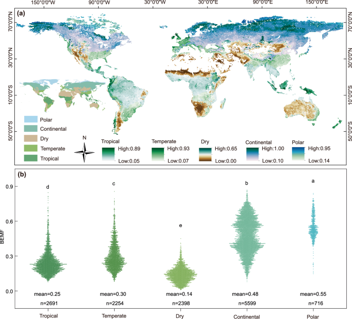
We used the Köppen–Geiger climate classification to discern whether there is a discrepancy of BEMF in different climate biomes. The global maps of the Köppen–Geiger climate classification were downloaded from figshare with a resolution of 1 km73. The Köppen climate classification is a system based on the regional temperature and precipitation. In detail, the tropics are warm and humid (MAT = 24.76 °C, MAP = 1689.67 mm), but the continental (MAT = −2.0 °C, MAP = 499.43 mm) and polar (MAT = −12.39 °C, MAP = 260.45 mm) biomes are relatively cold, and the dry biomes are dry (MAT = 18.30 °C, MAP = 267.13 mm).
Assessment of BEMF
The averaging, PCA, and single-threshold approaches were used to calculate the global maps of BEMF using ArcGIS Pro 3.1.5. The averaging approach has been consistently applied in previous research74. To ensure all ecosystem function data are in the same dimension, all ecosystem function data should be standardized before calculating. There are mainly two standardization methods of ecosystem function, namely, the Z-score method and the conversion method of maximum value. In our study, we calculated the standardized values using the Z-scores as described in the previous ref. 75, and the averaging approach collates the mean values of each standardized function in each 0.5° grid. The average approach is calculated as follows:
$${{\mbox{BEMF}}}_{{\mbox{average}}}=\frac{1}{F}\displaystyle {\sum }_{{\mbox{i}}=1}^{F}g({r}_{i}({\,\,f}_{i}))$$
(1)
where F represents the number of ecosystem functions; fi is the value of ecosystem function in ith; ri is a mathematical function that converts values to positive; g is a standardized treatment.
Compared to the averaging approach, the advantage of the PCA method is that it can reduce dimensions, prevent collinearity between indicators, and retain the information of each indicator76. Applying PCA does not involve the multiple contributions of correlated ecosystem functions77; the principal component axis in multifunctional space is calculated for fifteen standardized functions for each grid square. We then summed the PCA axis scores weighted by the degree of contribution of each axis into a single index to quantify BEMF. The PCA calculation method is as follows:
$${{\mbox{BEMF}}}_{{\mbox{PCA}}}=\displaystyle {\sum }_{i=1}^{n}{a}_{i}{{\mbox{PC}}}_{i}$$
(2)
where PCi is the ith principal component; αi is the contribution rate corresponding to the ith principal component; n is the total number of principal components selected. The first two principal components were used in our study, so n is equal to 2.
There is unprecedented heterogeneity of thresholds in each grid spanning a global scale that will lead to the calculation of global BEMF inapplicably using the multiple-threshold approach based on the ecosystem functions without time series; thus, we utilized the recommended method (the single-threshold) as described in the previous ref. 78. We employed the single-threshold to quantify BEMF and selected the 50% maximum for each ecosystem function as the threshold following the next two reasons: (1) If an ecosystem can provide 50% of the maximum species for a function, thereby considering that the ecosystem can maintain this function by referencing the median lethal effect concentration in ecotoxicology; (2) For any single function, on average one species was needed to maintain a specific process at ~60% of the maximum rate. Thus, selecting 50% as the threshold can maximize the probability, i.e., one function at least needs a species to sustain. It is important to note that the maximum represents the range at the top 5% of each ecosystem function, and that is to prevent outliers. After determining the threshold and maximum, we counted the total number of ecosystem functions that passed the prescribed threshold and thereby produced the global map of BEMF with the threshold approach. The single-threshold calculation method is as follows:
$${{{\mbox{BEMF}}}_{{\mbox{threshold}}}}=\displaystyle {\sum }_{i=1}^{F}\displaystyle {\sum }_{j=1}^{k}\left({r}_{ij}(\,\,{f}_{ij}) > {t}_{i}\right.$$
(3)
where F is the number of ecosystem functions; k is the total number of grid pixels of the ecosystem function. fij is the jth value of the ith ecosystem function; rij is a mathematical function that converts values to positive; ti is the ith ecosystem function threshold.
Although we used three basic approaches to assess worldwide BEMF, each approach has merits and demerits (Table S3)79,80. To address this issue, we averaged the three indexes after normalization to synthetically represent BEMF.
Similarity analysis of BEMF
We used two methods to examine the spatial similarity of BEMF using different approaches. To compare the similarity of BEMF, the comparison map profile (CMP) method was used, which employs the averaged values of cross-correlation coefficient (CC) and absolute distance (DD) from scales 1 (3 × 3 pixel moving window) to 10 (30 × 30 pixel moving window), their computational formula as follows81:
$${{\mbox{DD}}}={{abs}}(\bar{x}-\bar{y})$$
(4)
$${{\mbox{CC}}}=\frac{1}{{N}^{2}}{\sum }_{i=1}^{N}{\sum }_{j=1}^{N}\frac{({x}_{{ij}}-\bar{x})({y}_{{ij}}-\bar{y})}{{\sigma }_{x}{\sigma }_{y}}$$
(5)
$${\sigma }_{x}^{2}=\frac{1}{{N}^{2}-1}\displaystyle {\sum }_{i=1}^{N}\displaystyle {\sum }_{j=1}^{N}{({x}_{ij}-\bar{x})}^{2}$$
(6)
where \(\bar{x}\) and \(\bar{y}\) denote the averaged values of two moving windows for the two comparative images. xij and yij represent pixel values of two moving windows in two compared images in row i and column j, respectively. \({\sigma }_{x}\) and \({\sigma }_{y}\) denote the standard deviation corresponding to two moving windows of two comparative images. N is the pixel number of moving windows. Low DD and high CC values indicate more substantial similarity between two images, and vice versa. In addition, we used the Taylor Diagram and comparison map profile (CMP) to compare the similarity of BEMF based on the different approaches. This method is performed by the R 4.1.1 software (R Core Development Team, R Foundation for Statistical Computing, Vienna, Austria) using the “openair” package.
Global spatial patterns based on the three BEMF approaches (averaging, PCA, and single-threshold) are consistent (Fig. S16a–c), as shown by Taylor diagrams (all r > 0.75, standard deviation S17). Concordance correlation coefficient (CC) and discrepancy (DD) values indicate strong agreement between the averaging and PCA approaches (geometric mean CC = 0.64, geometric mean DD = 0.06; Fig. S18a, g), supporting the robustness of the PCA approach. Similarly, the averaging and threshold approaches show a strong correlation (geometric mean CC = 0.83, geometric mean DD = 0.06; Fig. S18b, h). However, the PCA and threshold approaches exhibit lower consistency (geometric mean CC = 0.31, geometric mean DD = 0.11; Fig. S18c, i), likely due to the discrete nature of the threshold approach. To address this discrepancy, we calculated the mean BEMF using the three approaches. This improves consistency between approaches in most areas (averaging-mean: geometric mean CC = 0.88, geometric mean DD = 0.06, Fig. S18d, j; PCA-mean: geometric mean CC = 0.52, geometric mean DD = 0.10, Fig. S18e, k; threshold-mean: geometric mean CC = 0.59, geometric mean DD = 0.10, Fig. S18f, l).
Data analyses
To eliminate the effects of differences in computing scale, we used log transformations to normalize the BEMF produced by the averaging, PCA, and single-threshold approaches. We averaged the BEMF calculated by the above three methods and further analyzed the BEMF through the following steps. Firstly, to explore the differences in BEMF between Köppen climate biomes (tropical, temperate, dry, continental, and polar), one-way ANOVAs with the Least Significant Difference (LSD) multiple comparisons were applied in R 4.1.1 software. Then, linear regression analysis was performed in SigmaPlot 10.0 (Systat Software, Inc., Chicago, IL, USA) to investigate relationships (R2) between the BEMF and climate (precipitation and temperature) across the Köppen climate biomes and globally, the computational formula as follows:
where Y is the dependent variable of BEMF; α is the coefficient between variables of Y and X; X represents the climate of precipitation or temperature; Y0 is a constant.
Secondly, given the strong correlation between temperature and BEMF at the global scale (Fig. 2a), piecewise linear regression fitting was conducted in SigmaPlot 10.0 to identify the existence of any thresholds, the computational formula as follows:
$$y=\left\{\begin{array}{l}\frac{{{{y}}}_{1}({{{T}}}_{1}-{{t}})+{{{y}}}_{2}({{t}}-{{{t}}}_{1})}{{{{T}}}_{{1}}-{{{t}}}_{1}},{{{t}}}_{1}\le {{t}}\le {{t{T}}}_{1}\\ \frac{{{{y}}}_{2}({{{t}}}_{2}-{{t}})+{{{y}}}_{3}({{t}}-{{{T}}}_{1})}{{{{t}}}_{2}-{{{T}}}_{1}},{{{T}}}_{1}\le {{t}}\le {{{t}}}_{{2}}\end{array}\right.$$
(8)
where y represents BEMF; t represents the climate of temperature; t1 is the minimum value of t; t2 is the maximum value of t; T1 repesents the threshold of MAT in our study; y1, y2, and y3 are the values of BEMF that corresponding to t1, T1, and t2, respectively.
Indeed, an abrupt change of BEMF was detected using this method at a MAT threshold of ~16.4 °C (Fig. 2b), and this figure was plotted using Origin 2024 (Origin Ro, Version 2024. OriginLab Corporation, Northampton, MA, USA). We then used linear regression analysis to evaluate the relationships between environmental factors of climate (MAT, and MAP), soil physical properties (pH, clay, and bulk density), as well as biodiversity properties (soil biodiversity, and plant species richness) and BEMF (Fig. 2 c, d), and plotted these figures by R 4.1.1 software with the packages of “ggplot2” and “gridExtra”. Meanwhile, if the absolute value of the coefficient of determination between the environmental factors and BEMF is >0.1, the factor can be considered an important determinant affecting BEMF, and further used in the SEM.
Thirdly, SEM was used to elucidate the direct and indirect relationships between BEMF, climate, soil properties, and biodiversity. An a priori structural equation modeling, based on previous studies1,4,7,8, hypothesized causal relationships among these factors (Fig. S19). Before modeling, correlations between BEMF and its indicators were assessed to identify key influential factors. The model was parameterized using the selected dataset in AMOS 21.0 (Amos Development Corporation, Chicago, IL, USA). Model fit was evaluated using the root mean square error of approximation (RMSEA; acceptable fit: 0.00 ≤ RMSEA ≤ 0.05), chi-squared test (χ2), and probability level (p; acceptable fit: p > 0.05)8.
Next, we assume that other factors (e.g., land-use, soil properties, and biodiversity) remain unchanged in the future to isolate the impact of climate change on BEMF. Our SEM results provide convincing evidence that temperature and precipitation primarily control BEMF in high and low BEMF patterns, respectively. Based on previous studies82,83,84,85, to screen machine learning models with high accuracy for simulating BEMF, four models (Random Forest, Boosted Regression Trees, Support Vector Machine, and Gradient Boosting Machine) were used in our study. We found that the Random Forest model exhibited high robustness and accuracy for predicting BEMF across both MAT ≤ 16.4 °C (high BEMF) and MAT > 16.4 °C (low BEMF) regions (Table S4). Consequently, we utilized the Random Forest model to simulate future BEMF changes under climate change scenarios. In detail, in both temperature-regulated and precipitation-regulated regions, the Random Forest algorithm was deployed to estimate BEMF and map its spatial patterns under three different future climate scenarios. SSP126 represents the sustainable development and low-emission pathway, SSP370 represents the imbalance development and intermediate emission pathway, and SSP585 represents the rapid development and high emission pathway86. Future bioclimatic data (MAT, mean diurnal range, isothermality, temperature seasonality, max temperature of warmest month, min temperature of coldest month, temperature annual range, mean temperature of wettest quarter, mean temperature of driest quarter, mean temperature of warmest quarter, and mean temperature of coldest quarter, MAP, precipitation of wettest month, precipitation of driest month, precipitation seasonality, precipitation of wettest quarter, precipitation of driest quarter, precipitation of warmest quarter, precipitation of coldest quarter) were obtained from the following ten models: ACCESS-CM2, CMCC-ESM2, EC-Earth3-Veg, GISS-E2-1-G, INM-CM5-0, IPSL-CM6A-LR, MIROC6, MPI-ESM1-2-HR, MRI-ESM2-0, and UKESM1-0-LL. In both temperature- and precipitation-regulated regions, the future bioclimatic data were divided into training (70%) and testing (30%) datasets. We configured the Random Forest regression model with 500 decision trees using the “randomForest” package in R software version 4.1.1. The model was then used to predict BEMF spatial patterns under the three different SSPs for two future periods (2021-2060 and 2061-2100). Model performance was evaluated using several metrics: correlation coefficient (CC), relative bias (BIAS), Nash–Sutcliffe coefficient efficiency (NSE), root mean square error (RMSE), and mean error (ME), calculated using test datasets. These metrics assessed the reliability of the predicted BEMF values. This comprehensive approach, leveraging extensive bioclimatic data and rigorous validation metrics, ensures the reliability and robustness of the Random Forest model in mapping BEMF under different climate scenarios.
Reporting summary
Further information on research design is available in the Nature Portfolio Reporting Summary linked to this article.