This study relies on the analysis of previously published data, adhering to ethical guidelines for human and mouse samples.
NicheCompass modelDataset
We define a spatial omics dataset as \({\mathcal{D}}=\{{{\bf{x}}}_{i},{{\bf{s}}}_{i},{{\bf{c}}}_{i},{{\bf{y}}}_{i}{\}}_{i=1}^{{N}_{\text{obs}}}\), where \({N}_{\text{obs}}\) is the total number of observations (cells or spots), \({{\bf{x}}}_{i}\in {{\mathbb{R}}}^{{N}_{\text{fts}}}\) is the omics feature vector, \({{\bf{s}}}_{i}\in {{\mathbb{R}}}^{2}\) is the 2D spatial coordinate vector, \({{\bf{c}}}_{i}\in {{\mathbb{N}}}^{{N}_{\mathrm{cov}}}\) is the label-encoded covariates vector (for example, sample or field of view) and \({{\bf{y}}}_{i}\in {{\mathbb{R}}}^{{N}_{\text{lbl}}}\) is the label vector (all vectors are row vectors). For unimodal data, \({{\bf{x}}}_{i}\) comprises raw gene expression counts such that \({{\bf{x}}}_{i}={{\bf{x}}}_{i}^{\left(\text{rna}\right)}\in {{\mathbb{R}}}^{{N}_{\text{rna}}}\), where \({N}_{\text{rna}}\) is the number of genes. For multimodal data, \({{\bf{x}}}_{i}\) combines raw gene expression counts and chromatin accessibility peak counts, such that \({{\bf{x}}}_{i}={{\bf{x}}}_{i}^{\left(\text{rna}\right)}{||}{{\bf{x}}}_{i}^{\left(\text{atac}\right)}\) (concatenation) with \({{\bf{x}}}_{i}^{\left(\text{atac}\right)}\in {{\mathbb{R}}}^{{N}_{\text{atac}}}\), where \({N}_{\text{atac}}\) is the number of peaks. We define corresponding matrices across observations with italic uppercase letters, for example, \({X}=\left[{{\bf{x}}_{1}}\right.\), …, \({{{\bf{x}}}_{{N}_{\text{obs}}}]}^{T}\in {{\mathbb{R}}}^{{N}_{\text{obs}}\times {N}_{\text{fts}}}\).
Neighborhood graph
We model the spatial structure of \({\mathcal{D}}\) using a neighborhood graph \({\mathcal{G}}=\left({\mathcal{V}},{\mathcal{E}},{{X}},{{Y}}\right)\), where each node \({{\mathcal{v}}}_{i}{\mathcal{\in }}{\mathcal{V}}\) represents an observation, each edge \(\left({{\mathcal{v}}}_{i},{{\mathcal{v}}}_{j}\right){\mathcal{\in }}{\mathcal{E}}\) indicates spatial neighbors, \({{\bf{x}}}_{i}\) is the attribute vector and \({{\bf{y}}}_{i}\) is the label vector of node \({{\mathcal{v}}}_{i}\). \({\mathcal{G}}\) is a disconnected graph composed of sample-specific, symmetric k-NN subgraphs \({{\mathcal{G}}}_{1}\), …, \({{\mathcal{G}}}_{{N}_{\text{spl}}}\) determined using Euclidean distances, where \({N}_{\text{spl}}\) is the number of samples. Using this strategy, we adapt to variable observation densities in tissue26, whereas alternative approaches, such as fixed-radius neighborhood graphs, can be used to consider local observation densities. We derive a spatial adjacency matrix \({A}\in {\{{0,1}\}}^{{N}_{\text{obs}}\times {N}_{\text{obs}}}\) from \({\mathcal{G}}\), where \({{{A}}}_{i,\,j}=1\) if \(\left({{\mathcal{v}}}_{i},{{\mathcal{v}}}_{j}\right){\mathcal{\in }}{\mathcal{E}}\) and \({{{A}}}_{i,\,j}=0\) otherwise.
Node labels
For each observation i, we define a neighborhood omics feature vector \({{{\bf{x}}}^{{\boldsymbol{{\prime} }}}}_{i}\):
$${{{\bf{x}}}^{{\boldsymbol{{\prime} }}}}_{i}=\sum _{j{\mathcal{\in }}{\mathcal{N}}\left(i\right)\cup \{i\}}\left[\frac{{{\bf{x}}}_{j}}{\sqrt{{d}_{j}{d}_{i}}}\right]$$
where \({d}_{i}\) denotes node degree, including a self-loop (\({d}_{i}={\sum }_{j{\mathcal{\in }}{\mathcal{N}}\left(i\right)\cup \left\{i\right\}}1\)). This aggregation combines node i’s omics feature vector with those of its neighbors \(j\in N\left(i\right)\), weighted by a graph convolution norm operator97. Self-loops model autocrine signaling, while neighboring nodes capture juxtacrine and paracrine signaling. Node labels are defined as \({{\bf{y}}}_{i}={{\bf{x}}}_{i}{||}{{{\bf{x}}}^{{\boldsymbol{{\prime} }}}}_{i}\).
Covariates
The covariates vector \({{\bf{c}}}_{i}\) models confounding effects. For multi-sample datasets, the sample ID (\({k}_{i}\)) is used as the first covariate (\({{\rm{C}}}_{i,1}={k}_{i}\)). Additional covariates, such as field of view and donor, are included if available to account for hierarchical effects. We further introduce a one-hot-encoded notation of covariate vectors with each covariate \(l=1,\) …, \({N}_{\mathrm{cov}}\) represented by a separate vector \({{\bf{c}}}_{i}^{\left(l\right)}\in \{\mathrm{0,1}{\}}^{{N}_{{\text{cat}}^{\left(l\right)}}}\), where \({N}_{{\text{cat}}^{\left(l\right)}}\) is the number of unique categories of covariate \(l\). Given that \({\mathcal{G}}\) is composed of sample-specific subgraphs, some covariates (for example, sample, donor) are tied to connected components. We denote such covariates as pure (\({L}_{\rm{p}}\)), while covariates that vary within components (for example, field of view) are denoted as mixed (\({L}_{\rm{m}}\)).
Gene programs
Prior programs are represented by two binary program gene matrices \({P}^{\left({\text{pr}},{\text{rna}}\right)},{P}^{{\prime} \left({\text{pr}},{\text{rna}}\right)}\in {\{{0,1}\}}^{{N}_{\text{pr}}\times {N}_{\text{rna}}}\), where \({N}_{\text{pr}}\) is the number of prior programs. \({{{P}}}^{\left({\text{pr}},{\text{rna}}\right)}\) indicates genes in the self component, while \({{{P}}}^{{\prime} \left(\text{pr},\text{rna}\right)}\) indicates genes in the neighborhood component. For multimodal data, two additional binary program peak matrices, \({{{P}}}^{\left({\text{pr}},{\text{atac}}\right)}\) and \({{{P}}}^{{\prime} \left({\text{pr}},{\text{atac}}\right)}\in {\{{0,1}\}}^{{N}_{\text{pr}}\times {N}_{\text{atac}}}\), capture peaks linked to genes in the self components and neighborhood components, respectively. \({{{P}}}^{\left({\text{pr}},{\text{rna}}\right)}\) and \({{{P}}}^{{\prime} \left({\text{pr}},{\text{rna}}\right)}\) must be provided to NicheCompass by in-built database APIs or custom user inputs. By default, \({{{P}}}^{\left({\text{pr}},{\text{atac}}\right)}\) and \({{{P}}}^{{\prime} \left({\text{pr}},{\text{atac}}\right)}\) are derived from program gene matrices by associating peaks overlapping gene bodies or promoter regions (up to 2,000 bp upstream of transcription start sites); however, users can customize these to represent specific regulatory networks. De novo programs are analogously defined by binary matrices \({{{P}}}^{\left({\text{nv}},{\text{rna}}\right)}\), \({{{P}}}^{{\prime} \left({\text{nv}},{\text{rna}}\right)}\in {\{{0,1}\}}^{{N}_{\text{nv}}\times {N}_{\text{rna}}}\) and, for multimodal data, \({{{P}}}^{\left({\text{nv}},{\text{atac}}\right)}\) and \({{{P}}}^{{\prime} \left({\text{nv}},{\text{atac}}\right)}\in {\{{0,1}\}}^{{N}_{\text{nv}}\times {N}_{\text{atac}}}\), where \({N}_{\text{nv}}\) is the number of de novo programs (default, \({N}_{\text{nv}}=100\)). In \({{{P}}}^{\left({\text{nv}},{\text{rna}}\right)}\) and \({{{P}}}^{{\prime} \left({\text{nv}},{\text{rna}}\right)}\), elements are set to 1 for genes not included in the respective self or neighborhood components of prior programs. In peak matrices, elements are set to 1 for peaks linked to genes. The total number of programs is \({N}_{\text{gp}}={N}_{\text{pr}}+{N}_{\text{nv}}\).
Default prior programs
NicheCompass provides default prior programs through APIs with interaction databases. For cell–cell-communication programs, ligand–receptor interactions are retrieved from OmniPath37 and metabolite-sensor interactions from MEBOCOST38. For transcriptional regulation programs, transcription factors and their downstream genes are retrieved from CollecTRI42 through decoupler40. For combined interaction programs, NicheNet’s regulatory potential matrix (V2)39, consisting of ligands, receptors and downstream target genes, is used. As recommended by MultiNicheNet41, programs are filtered to include at most 250 target genes, ranked by regulatory score. In our experiments, we filtered subsets within prior programs and merged programs if they shared at least 90% source and target genes. This resulted in 2,925 (2,904) mouse (human) prior programs, including 548 (490) ligand–receptor programs, 114 (116) metabolite-sensor programs, 1,286 (1,225) combined interaction programs and 977 (1,073) transcriptional regulation programs (the latter were only included in multimodal scenarios).
Model overview
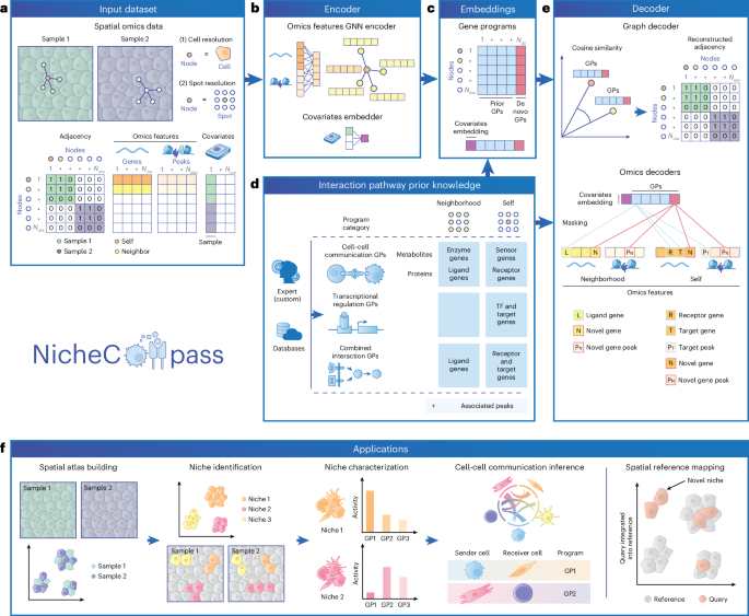
NicheCompass extends the variational graph autoencoder framework48 to enable interpretable, scalable and integrative modeling of spatial multi-omics data. The model includes a graph encoder and a multi-module decoder, trained in a self-supervised, multi-task learning setup with node-level and edge-level tasks. The decoder comprises a graph decoder to reconstruct \({{A}}\) from \({{Z}}\) and two omics decoders per modality: a self-omics decoder to reconstruct modality-specific features \({{{X}}}^{\left({\mathrm{mod}}\right)}\) and a neighborhood omics decoder to reconstruct neighborhood features \({{{X}}}^{{{{\prime} }}\left({\mathrm{mod}}\right)}\). This ensures embeddings \({{Z}}\) integrate spatial information from \({\mathcal{G}}\) and molecular information from \({{X}}\) and \({{{X}}}^{{{{\prime} }}}\), thus providing spatially and molecularly consistent embeddings \({{\bf{z}}}_{i}\in {{\mathbb{R}}}^{{N}_{\text{gp}}}\) for each observation i. Program matrices are used to mask the reconstruction of \({{X}}\) and \({{{X}}}^{{{{\prime} }}}\), ensuring each feature \(u\) in \({{\bf{Z}}}_{:,u}\) represents a spatial program. Embeddings for prior programs are denoted as \({{{Z}}}^{\left({\text{pr}}\right)}\in {{\mathbb{R}}}^{{N}_{\text{obs}}\times {N}_{\text{pr}}}\) and those for de novo programs are denoted as \({{{Z}}}^{\left({\text{nv}}\right)}\in {{\mathbb{R}}}^{{N}_{\text{obs}}\times {N}_{\text{nv}}}\), with \({{\bf{z}}}_{i}={{\bf{z}}}_{i}^{\left(\text{pr}\right)}{||}{{\bf{z}}}_{i}^{\left(\text{nv}\right)}\). Following the variational autoencoder standard, we use a standard normal prior for the latent variables \({{Z}}_{u}^{\left(i\right)}{\mathcal{\sim }}{\mathcal{N}}\left({0,1}\right)\) and apply the reparameterization trick to enable end-to-end training by backpropagation.
Encoder
The first layer of the graph encoder is fully connected with hidden size \({N}_{\text{hid}}={N}_{\text{gp}}\), serving two purposes: learning internal cell or spot representations from the full omics feature vector \({{\bf{x}}}_{i}\) before neighborhood aggregation and reducing the dimensionality of \({{\bf{x}}}_{i}\) when \({N}_{\text{fts}}\) > \({N}_{\text{gp}}\). This layer is followed by two parallel message-passing layers that compute the mean (\({{\mathbf{\upmu }}}_{i}\)) and log standard deviation (\(\log \left({{\mathbf{\upsigma }}}_{i}\right)\)) vectors of the variational posterior, where \({{\mathbf{\upmu }}}_{i}\) is extracted as cell embedding vector \({{\bf{z}}}_{i}\). The default model uses graph attention layers with dynamic attention98 (\({N}_{\text{head}}=4\)); in NicheCompass Light, graph convolutional layers replace graph attention layers (Supplementary Methods). Additionally, the model learns an embedding matrix \({{{W}}}^{\left({\text{emb}}{\_}{e}^{\left(l\right)}\right)}\in {{\mathbb{R}}}^{{N}_{\text{emb}}\times {N}_{{\text{cat}}^{\left(l\right)}}}\) for each covariate \(l\), where \({N}_{\text{emb}}\) is the embedding size, to retrieve an embedding vector \({{\bf{e}}}_{i}^{\left(l\right)}\) from the one-hot-encoded vector representation \({{\bf{c}}}_{i}^{\left(l\right)}\). The final covariate embedding is \({{\bf{e}}}_{i}={{\bf{e}}}_{i}^{\left(1\right)}{||}\cdots {||}{{\bf{e}}}_{i}^{\left({N}_{\mathrm{cov}}\right)}\in {{\mathbb{R}}}^{{N}_{\text{emb}}}\).
Decoder
The graph decoder reconstructs \({{A}}\) using cosine similarity between node embeddings, restricted to nodes with identical pure categorical covariates (for example, same sample):
\(\displaystyle{\widetilde{{\rm{A}}}}_{i,\,j}=\displaystyle\text{cosine similarity}\left({{\bf{z}}}_{i},{{\bf{z}}}_{j}\right)=\displaystyle\frac{{{\bf{z}}}_{i}\cdot {{\bf{z}}}_{j}}{\left|{{\bf{z}}}_{i}\right|\left|{{\bf{z}}}_{j}\right|}\)
Omics decoders reconstruct node labels \({{Y}}\) by estimating mean parameters \({\varPhi }_{i,\,f},{\varPhi }_{i,\,f}^{{\prime} }\) of negative binomial distributions that generate omics features (\({{X}}_{f}^{\left(i\right)}{\mathcal{\sim }}{\mathcal{N}}{\mathcal{B}}\left({\varPhi }_{i,f},{\theta }_{f}\right)\) and \({{X}}_{f}^{{\prime} \left(i\right)}{\mathcal{\sim }}{\mathcal{N}}{\mathcal{B}}\left({\varPhi }_{i,\,f,}^{{\prime}}{\theta }_{f}^{{\prime} }\right)\), where \(f\) is an omics feature, \({{X}}^{\left(i\right)}\) and \({{X}}^{{\prime} \left(i\right)}\) are random variables and \({\theta }_{f},{\theta }_{f}^{{\prime} }\) represent inverse dispersion parameters). They are composed of modality-specific single-layer linear decoders such that each embedding feature \(u\) in \({{Z}}_{:,u}^{\left(\text{pr}\right)}\) is incentivized to learn the activity of a specific prior program. This is achieved by prior program matrices (\({{{P}}}^{\left({\text{pr}},{\text{rna}}\right)}\), \({{{P}}}^{{\prime} \left({\text{pr}},{\text{rna}}\right)}\), \({{{P}}}^{\left({\text{pr}},{\text{atac}}\right)}\), \({{{P}}}^{{\prime} \left({\text{pr}},{\text{atac}}\right)}\)) constraining decoder contributions to specific genes or peaks. For instance, if \({{{P}}}_{u,q}^{\left({\text{pr}},{\text{rna}}\right)}=1\), embedding feature \({{Z}}_{:,u}\) contributes to reconstructing gene \(q\) in the self component. Similar logic applies to neighborhood components and multimodal features. \({{{Z}}}_{i,u}\) can therefore be interpreted as observation i’s representation of program \(u\), where the self component of \(u\) is composed of all genes \(q\) and peaks \(s\) for which \({{{P}}}_{u,q}^{\left({\text{pr}},{\text{rna}}\right)}=1\) and \({{{P}}}_{u,s}^{\left({\text{pr}},{\text{atac}}\right)}=1\), and its neighborhood component of all genes \(r\) and peaks \(t\) for which \({{{P}}}_{u,r}^{{\prime} \left({\text{pr}},{\text{rna}}\right)}=1\) and \({{{P}}}_{u,t}^{{\prime} \left({\text{pr}},{\text{atac}}\right)}=1\). De novo programs are similarly masked using \({{{P}}}^{\left({\text{nv}},{\text{rna}}\right)},{{{P}}}^{\left({\text{nv}},{\text{atac}}\right)},{{{P}}}^{{\prime} \left({\text{nv}},{\text{rna}}\right)}\) and \({{{P}}}^{{\prime} \left({\text{nv}},{\text{atac}}\right)}\), allowing them to reconstruct omics features not included in prior knowledge. Confounding effects are removed by injecting covariate embeddings \({{\bf{e}}}_{i}\) into omics decoders. For observation i, the reconstructed mean parameter is:
$$\begin{array}{l}{{{\phi }}}_{i}^{* \left(\mathrm{mod}\right)}=\text{Softmax}\left({{{P}}}^{{\left(\text{pr},\mathrm{mod}\right)}^{T}}\circ {{{W}}}^{\left({\text{pr}{\_}}{\phi }^{* \left(\mathrm{mod}\right)}\right)}{{\bf{z}}}_{i}^{\rm{pr}}\right.\\\left.+\,{{{P}}}^{{\left(\text{nv},\mathrm{mod}\right)}^{T}}\circ {{{W}}}^{\left({\text{nv}{\_}}{\phi }^{* \left(\mathrm{mod}\right)}\right)}{{\bf{z}}}_{i}^{\rm{nv}}+{{{W}}}^{\left({\text{emb}{\_}}{\phi }^{* \left(\mathrm{mod}\right)}\right)}{{\bf{e}}}_{i}\right)\exp \left({{{\upiota }}}_{{\mathcal{i}}}^{* \left(\mathrm{mod}\right)}\right)\end{array}$$
where * indicates either the self component or neighborhood component, \(\mathrm{mod}\) represents the modality (rna or atac), \({{\upiota }_{{\mathcal{i}}}^{* \left(\mathrm{mod}\right)}}\) is the empirical log library size and \({{{W}}}^{\left({\text{pr}}{\_}{\phi }^{* \left({\mathrm{mod}}\right)}\right)}\in {{\mathbb{R}}}^{{N}_{\mathrm{mod}}\times {N}_{\text{pr}}}\), \({{{W}}}^{\left({\text{nv}}{\_}{\phi }^{* \left({\mathrm{mod}}\right)}\right)}\in {{\mathbb{R}}}^{{N}_{{\mathrm{mod}}}\times {N}_{\text{nv}}}\) and \({{{W}}}^{\left({\text{emb}}{\_}{\phi }^{* \left({\mathrm{mod}}\right)}\right)}\in {{\mathbb{R}}}^{{N}_{\mathrm{mod}}\times {N}_{\text{emb}}}\) are learnable weights. The Softmax activation operates across features, constraining omics decoders to output mean proportions. The multiplication with the empirical library size ensures the same size factors as in the input domain.
Neighbor sampling data loaders
NicheCompass uses mini-batch training with inductive neighbor sampling data loaders99 for scalability and efficiency. For each node \({{\mathcal{v}}}_{i}{\mathcal{\in }}{\mathcal{V}}\), only \({n}=4\) sampled neighbors from \({\mathcal{G}}\) are used for message passing. NicheCompass’ multi-task architecture uses two data loaders: a node-level loader to reconstruct \({{X}}\) and \({{{X}}}^{{\boldsymbol{{\prime} }}}\) and an edge-level loader to reconstruct \({{A}}\). One iteration of the model includes one forward pass per loader and a joint backward pass for simultaneous gradient computation. For the node-level loader, a batch consists of \({N}_{{{\mathcal{V}}}_{\text{bat}}}\) randomly selected nodes \({{\mathcal{V}}}_{\,{\text{bat}}}{\mathcal{\in }}{\mathcal{V}}\), shuffled at each iteration. For the edge-level loader, a batch includes \({N}_{{{\mathcal{E}}}_{\text{bat}}}\) positive node pairs \(\left(i,j\right){\mathcal{\in }}{\mathcal{E}}\), shuffled per iteration, and an equal number of randomly sampled negative pairs \(\left(i,j\right)\) for which \({{{A}}}_{i,\,j}=0\). We denote the corresponding batch of positive and sampled negative node pairs as \({{\mathcal{E}}}_{\text{bat}}\). To ensure valid negative examples, we retain only node pairs that share identical pure covariates (\({{\bf{c}}}_{i}^{\left(l\right)}={{\bf{c}}}_{j}^{\left(l\right)}\forall l\in {L}_{\rm{p}}\)). The final edge batch \({{\mathcal{E}}}_{\rm{rec}}=\{{{\mathcal{E}}}_{\rm{rec}}^{+},{{\mathcal{E}}}_{\rm{rec}}^{-}\}\) consists of positive pairs \({{\mathcal{E}}}_{\rm{rec}}^{+}=\{\left(i,j\right)\in {{\mathcal{E}}}_{\text{bat}}{\rm{| }}{{{A}}}_{i,\,j}=1\}\) and valid negative pairs \({{\mathcal{E}}}_{\rm{rec}}^{-}=\{\left(i,j\right)\in {{\mathcal{E}}}_{\text{bat}}{\rm{| }}{{{A}}}_{i,j}=0\) and \({{\bf{c}}}_{i}^{\left(l\right)}={{\bf{c}}}_{j}^{\left(l\right)}\forall l\in {L}_{\rm{p}}\}\).
Program pruning
To prioritize relevant programs, NicheCompass uses a dropout-based pruning mechanism. This addresses issues with overlapping genes across programs that dilute correlations between embeddings \({{Z}}\) and program member genes. After a warm-up period, pruning is based on each program’s contribution to reconstructing \({{{X}}}^{\left(\text{rna}\right)}\) and \({{{X}}}^{{\boldsymbol{{\prime} }}\left(\text{rna}\right)}\). Contributions (\({\delta }_{u}\)) are calculated by aggregating absolute values of gene expression decoder weights at the program level (across self and neighborhood components) and scaling them by an estimate of the mean absolute embeddings across observations. This estimate is obtained as the exponential moving average of batch-wise forward passes. The maximum contribution (\({\delta }_{\max }\)) serves as a reference, and programs with contributions below a threshold (\(\tau * {\delta }_{\max }\), where \(\tau\) is a hyperparameter) are dropped. To balance pruning, two aggregation methods are used: sum-based (to avoid penalizing programs with many unimportant but few very important genes) and non-zero mean-based (to prevent prioritizing programs with many genes). Pruning is applied separately to prior and de novo programs, with independent \({\delta }_{\max }\) calculations.
Program regularization
To prioritize critical genes within programs while considering different functional importances (for example, a ligand is critical for the pathway), NicheCompass uses selective regularization. Genes in prior programs are categorized (ligand, receptor, transcription factor, sensor, target gene), and an L1 regularization loss is applied to decoder weights of specified categories. In our analyses, regularization was applied to target genes. De novo programs, which may include hundreds to thousands of genes, are similarly regularized with an L1 loss to encourage specificity. If decoder weights for gene expression are regularized to zero, corresponding weights for chromatin accessibility are set to zero, effectively deactivating those peaks within the program.
Loss function
With unimodal data, the loss function consists of four components: (1) a binary cross-entropy loss for reconstructing edges in \({{A}}\); (2) a negative binomial loss for reconstructing the self component \({{{X}}}^{\left(\text{rna}\right)}\); that is, the nodes’ gene expression counts; (3) a negative binomial loss for reconstructing the neighborhood component \({{{X}}}^{{\prime} \left(\text{rna}\right)}\); that is, the aggregated gene expression counts of node neighborhoods; and (4) the Kullback–Leibler divergence between variational posteriors and standard normal priors for latent variables. In multimodal scenarios, additional negative binomial losses are included for reconstructing self (\({{{X}}}^{\left(\text{atac}\right)}\)) and neighborhood peak counts (\({{{X}}}^{{\prime} \left(\text{atac}\right)}\)). The mini-batch-wise formulation of the edge reconstruction loss is:
$$\begin{array}{l}{{\mathcal{L}}}^{\left(\text{edge}\right)}\left(\widetilde{{{A}}};{{A}},{{\mathcal{E}}}_{\rm{rec}}\right)=-\frac{1}{\left|{{\mathcal{E}}}_{\rm{rec}}\right|}\sum _{\left(i,\,j\,\right)\in {{\mathcal{E}}}_{\rm{rec}}}\left[{\omega }_{\rm{pos}}{{{A}}}_{i,\,j}{\rm{log}}\left({\sigma} \left({\widetilde{{{A}}}}_{i,\,j}\right)\right)\right.\\\left.\qquad\qquad\qquad\qquad\quad+\,\left(1-{{{A}}}_{i,\,j}\right){\rm{log}}\left(1-\sigma \left({\widetilde{{{A}}}}_{i,\,j}\right)\right)\right].\end{array}$$
where \(\widetilde{{{A}}}\) represents edge reconstruction logits computed by the cosine similarity graph decoder. To balance the contribution of positive and negative edge pairs, a weight \({\omega }_{\rm{pos}}=\frac{\left|{{\mathcal{E}}}_{\rm{rec}}^{-}\right|}{\left|{{\mathcal{E}}}_{\rm{rec}}^{+}\right|}\) is applied as \(\left|{{\mathcal{E}}}_{\rm{rec}}^{+}\right|\ge \left|{{\mathcal{E}}}_{\rm{rec}}^{-}\right|\), owing to filtering negative pairs where pure covariates differ.
The mini-batch-wise formulation of the modality-specific omics reconstruction losses is:
$$\begin{array}{l}\displaystyle{{\mathcal{L}}}^{\left({\mathrm{mod}}\right)}\left({{{\varPhi }}}^{\left({\mathrm{mod}}\right)},{{{\varPhi }}}^{{\prime} \left({\mathrm{mod}}\right)},{{\mathbf{\uptheta }}}^{\left({\mathrm{mod}}\right)},{{\mathbf{\uptheta }}}^{{\prime} \left({\mathrm{mod}}\right)};{{{X}}}^{\left({\mathrm{mod}}\right)},{{{X}}}^{{\prime} \left({\mathrm{mod}}\right)},{{\mathcal{V}}}_{\,{{\text{bat}}}}\right)\\=\displaystyle\frac{1}{{N}_{{{\mathcal{V}}}_{\text{bat}}}}\sum _{i\in {{\mathcal{V}}}_{\text{bat}}}{{\mathcal{L}}}_{i}^{\left({\mathrm{mod}}\right)}\left({{\mathbf{\upphi }}}_{i}^{\left({\mathrm{mod}}\right)},{{\mathbf{\upphi }}}_{i}^{{\prime} \left({\mathrm{mod}}\right)},{{\mathbf{\uptheta }}}^{\left({\mathrm{mod}}\right)},{{\mathbf{\uptheta }}}^{{\prime} \left({\mathrm{mod}}\right)};{{\bf{x}}}_{i}^{\left({\mathrm{mod}}\right)},{{\bf{x}}}_{i}^{{\prime} \left({\mathrm{mod}}\right)}\right)\end{array}$$
where the observation-level loss includes the self component and neighborhood component negative binomial losses (Supplementary Methods):
$$\begin{array}{l}{{\mathcal{L}}}_{i}^{\left(\mathrm{mod}\right)}\left({{\mathbf{\upphi }}}_{i}^{\left({\mathrm{mod}}\right)},{{\mathbf{\upphi }}}_{i}^{{\prime} \left({\mathrm{mod}}\right)},{{\mathbf{\uptheta }}}^{\left({\mathrm{mod}}\right)},{{\mathbf{\uptheta }}}^{{\prime} \left({\mathrm{mod}}\right)};{{\bf{x}}}_{i}^{\left({\mathrm{mod}}\right)},{{\bf{x}}}_{i}^{{\prime} \left({\mathrm{mod}}\right)}\right)\\=\text{NBL}\left({{\mathbf{\upphi }}}_{i}^{\left({\mathrm{mod}}\right)},{{\mathbf{\uptheta }}}^{\left({\mathrm{mod}}\right)};{{\bf{x}}}_{i}^{\left({\mathrm{mod}}\right)}\right)+{\text{NBL}}\left({{\mathbf{\upphi }}}_{i}^{{\prime} \left({\mathrm{mod}}\right)},{{\mathbf{\uptheta }}}^{{\prime} \left({\mathrm{mod}}\right)};{{\bf{x}}}_{i}^{{\prime} \left({\mathrm{mod}}\right)}\right)\end{array}$$
where \(\mathrm{mod}\) represents the modality, \({{\mathbf{\uptheta }}}^{* \left({\mathrm{mod}}\right)}\) are feature-specific learned inverse dispersion parameters and \({{\mathbf{\upphi }}}_{i}^{* \left({\mathrm{mod}}\right)}\) are the estimated means, retrieved as output of the omics decoders.
The L1 regularization losses are defined as:
$${{\mathcal{L}}}^{\left({\text{L}}1,{\text{pr}}\right)}\left({{{W}}}^{\left({\text{pr}}{\_}{\phi }^{* \left({\text{rna}}\right)}\right)}\right)=\mathop{\sum }\limits_{u=1}^{{N}_{\text{pr}}}\mathop{\sum }\limits_{q=1}^{{N}_{\text{rna}}}\left|{{{W}}}_{q,u}^{\left({\text{pr}}{\_}{\phi }^{* \left({\text{rna}}\right)}\right)}\right|\circ {{{I}}}_{q,u}^{\left({\text{pr}}{\_}{\phi }^{* \left({\text{rna}}\right)}\right)}$$
and
$${{\mathcal{L}}}^{\left({\text{L}}1,{\text{nv}}\right)}\left({{{W}}}^{\left({\text{nv}}{\_}{\phi }^{* \left({\text{rna}}\right)}\right)}\right)=\mathop{\sum }\limits_{u=1}^{{N}_{\text{nv}}}\mathop{\sum }\limits_{q=1}^{{N}_{\text{rna}}}\left|{{{W}}}_{q,u}^{\left({\text{nv}}{\_}{\phi }^{* \left({\text{rna}}\right)}\right)}\right|$$
where \({{{I}}}^{\left({\text{pr}}{\_}{\phi }^{* \left({\text{rna}}\right)}\right)}\in {\{{0,1}\}}^{{N}_{\text{rna}}\times {N}_{\text{pr}}}\) is an indicator matrix for selective regularization of prior programs, with an entry of 1 indicating that the corresponding gene is part of a regularized category.
The mini-batch-wise formulation of the KL divergence consists of node-level and edge-level components:
$$\begin{array}{c}{{\mathcal{L}}}^{\left({\text{KL}}\right)}\left({{M}},{{{\varSigma}}};{{X}},{{\mathcal{V}}}_{\text{bat}},{{\mathcal{E}}}_{\text{bat}}\right)=\\ \frac{1}{{N}_{{{\mathcal{V}}}_{\text{bat}}}}\mathop{\sum}\limits_{i\in {{\mathcal{V}}}_{\text{bat}}}{{\mathcal{L}}}_{i}^{\left({\text{KL}}\right)}\left({{\mathbf{\upmu }}}_{i},{{\mathbf{\upsigma }}}_{i};{{\bf{x}}}_{{\bf{i}}}\right)\\+\frac{1}{4* {N}_{{{\mathcal{E}}}_{\text{bat}}}}\mathop{\sum}\limits_{\left(i,\,j\,\right)\in {{\mathcal{E}}}_{\text{bat}}}{{\mathcal{L}}}_{i}^{\left({\text{KL}}\right)}\left({{\mathbf{\upmu }}}_{i},{{\mathbf{\upsigma }}}_{i};{{\bf{x}}}_{{{i}}}\right)+{{\mathcal{L}}}_{j}^{\left({\text{KL}}\right)}\left({{\mathbf{\upmu }}}_{j},{{\mathbf{\upsigma }}}_{j};{{\bf{x}}}_{{\bf{j}}}\right)\end{array}$$
with the observation-level loss:
$$\begin{array}{l}{{\mathcal{L}}}_{i}^{\left({\text{KL}}\right)}\left({{\mathbf{\upmu }}}_{i},{{\mathbf{\upsigma }}}_{i};{{\bf{x}}}_{{\bf{i}}}\right)={D}_{\text{KL}}\left({q}_{{{\mathbf{\upmu }}}_{i},{{\mathbf{\upsigma }}}_{i}}\left({{Z}}^{\left(i\right)}|{{X}}^{\left(i\right)}\right)\parallel p\left({{Z}}^{\left(i\right)}\right)\right)\\\qquad\qquad\qquad\qquad=\,\displaystyle-\frac{1}{2}\mathop{\sum }\limits_{u=1}^{{N}_{\rm{gp}}}\left[1+\log \left({\mathbf{\upsigma} }_{{i}_{u}}^{2}\right)-{\mathbf{\upmu} }_{{i}_{u}}^{2}-{\mathbf{\upsigma} }_{{i}_{u}}^{2}\right]\end{array}$$
where \({{\mathbf{\upmu }}}_{i}\) and \({{\mathbf{\upsigma }}}_{i}\) are the estimated mean and standard deviation of the variational posterior normal distribution.
The final mini-batch loss combines all components:
$$\begin{array}{c}{\mathcal{L}}\left({{M}},{{\varSigma }},{\varPhi},{\varPhi}^{{\prime} },{\mathbf{\uptheta }},{{\mathbf{\uptheta }}}^{{\prime} },\widetilde{{{A}}},{{{W}}}^{\left({\text{rna}}\right)};{{A}},{{X}},{{{X}}}^{\prime},{{\mathcal{V}}}_{\,{\text{bat}}},{{\mathcal{E}}}_{\text{bat}}\right)\\={{\mathcal{L}}}^{\left({\text{KL}}\right)}\left({{M}},{{\Sigma }};{{X}},{{\mathcal{V}}}_{\text{bat}},{{\mathcal{E}}}_{\text{bat}}\right)\\+\,{\lambda }^{\left({\text{edge}}\right)}{{\mathcal{L}}}^{\left({\text{edge}}\right)}\left(\widetilde{{{A}}};{{A}},{{\mathcal{E}}}_{\rm{rec}}\right)\\+\,{\lambda }^{\left({\text{rna}}\right)}{{\mathcal{L}}}^{\left({\text{rna}}\right)}\left({{{\varPhi }}}^{\left({\text{rna}}\right)},{{{\varPhi }}}^{{\prime} \left({\text{rna}}\right)},{{\mathbf{\uptheta }}}^{\left({\text{rna}}\right)},{{\mathbf{\uptheta }}}^{{\prime} \left({\text{rna}}\right)};{{{X}}}^{\left({\text{rna}}\right)},{{{X}}}^{{\prime} \left({\text{rna}}\right)},{{\mathcal{V}}}_{\,{\text{bat}}}\right)\\+{\lambda }^{\left({\text{atac}}\right)}{{\mathcal{L}}}^{\left({\text{atac}}\right)}\left({{{\varPhi }}}^{\left({\text{atac}}\right)},{{{\varPhi }}}^{{\prime} \left({\text{atac}}\right)},{{\mathbf{\uptheta }}}^{\left({\text{atac}}\right)},{{\mathbf{\uptheta }}}^{{\prime} \left({\text{atac}}\right)};{{{X}}}^{\left({\text{atac}}\right)},{{{X}}}^{{\prime} \left({\text{atac}}\right)},{{\mathcal{V}}}_{\,{\text{bat}}}\right)\\+{\lambda }^{\left({\text{L}}1,{\text{pr}}\right)}{{\mathcal{L}}}^{\left({\text{L}}1,{\text{pr}}\right)}\left({{{W}}}^{\left({\text{pr}}{\_}{\phi }^{\left({\text{rna}}\right)}\right)}\right)\\+{\lambda }^{\left({\text{L}}1,{\text{pr}}\right)}{{\mathcal{L}}}^{\left({\text{L}}1,{\text{pr}}\right)}\left({{{W}}}^{\left({\text{pr}}{\_}{\phi }^{{\prime} \left({\text{rna}}\right)}\right)}\right)\\+{\lambda }^{\left({\text{L}}1,{\text{nv}}\right)}{{\mathcal{L}}}^{\left({\text{L}}1,{\text{nv}}\right)}\left({{{W}}}^{\left({\text{nv}}{\_}{\phi }^{\left({\text{rna}}\right)}\right)}\right)\\+{\lambda }^{\left({\text{L}}1,{\text{nv}}\right)}{{\mathcal{L}}}^{\left({\text{L}}1,{\text{nv}}\right)}\left({{{W}}}^{\left({\text{nv}}{\_}{\phi }^{{\prime} \left({\text{rna}}\right)}\right)}\right)\end{array}$$
where \(\lambda\) values denote weighting factors.
Spatial reference mapping
To map unseen query datasets onto spatial reference atlases, we use weight-restricted fine-tuning inspired by architectural surgery95. A NicheCompass model is first trained to construct a reference. During query training, all weights are frozen except for covariate embedding matrices (\({{{W}}}^{\left({\text{emb}}{\_}{e}^{\left(l\right)}\right)}\)), allowing us to capture query-specific variation without catastrophic forgetting. Programs can be pruned differently during query training owing to updating exponential moving averages of embeddings.
Program feature importances
Gene and peak importances for each program are determined using the learned weights of omics decoders. Absolute values of the gene expression or chromatin accessibility decoder weights are normalized across genes or peaks in the self and neighborhood components, ensuring that the importances sum to 1 per program.
Program activities
NicheCompass embeddings quantify pathway activity in cells or spots but are agnostic to sign. To ensure positive embedding values represent upregulation, the embeddings are adjusted based on omics decoder weight signs. For prior programs, embeddings are reversed if the aggregated weight of source genes (or target genes if source genes are absent) is negative. For de novo programs, the sign is reversed if the aggregated weight of all genes is negative. These sign-corrected embeddings are referred to as program activities.
Differential testing of program activities
We test differential program activity between groups of interest using the logarithm of the Bayes factor (\(\log K\)), a Bayesian generalization of the P value100. The hypothesis \({H}_{0}:{{\mathbb{E}}}_{a}\left[{{Z}}_{u}^{\left(a\right)}\right] > {{\mathbb{E}}}_{b}\left[{{Z}}_{u}^{\left(b\right)}\right]\) is tested against \({H}_{1}:{{\mathbb{E}}}_{a}\left[{{Z}}_{u}^{\left(a\right)}\right]\le {{\mathbb{E}}}_{b}\left[{{Z}}_{u}^{\left(b\right)}\right]\), where \(u\) is the program index, and \({{Z}}^{\left(a\right)}\) and \({{Z}}^{\left(b\right)}\) denote random variables for the program activities of group \(a\) and comparison group \(b\). The test statistic, \(\log K=\log \frac{p\left({H}_{0}\right)}{p\left({H}_{1}\right)}=\log \frac{p\left({H}_{0}\right)}{1-p\left({H}_{0}\right)}\), quantifies the evidence for \({H}_{0}\) (Supplementary Methods). Programs with \(\left|\log K\right|\ge 2.3\) are considered differentially expressed, corresponding to strong evidence101, equivalent to a relative ratio of probabilities of \(\exp \left(2.3\right)\approx 10\).
Selection of characterizing niche programs
To identify characterizing programs, we first perform a one-vs-rest differential log Bayes factor test to determine enriched programs. From these, we select two programs per niche based on the correlation between program activities and the expression of the program’s important target genes and ligand-encoding and receptor-encoding or enzyme-encoding and sensor-encoding genes.
Program communication potential scores
To compute source and target communication potential scores, we first scale gene expression between 0 and 1 to avoid bias towards highly expressed genes. For each program, the scaled expression of each member gene is multiplied by its corresponding omics decoder weight, yielding program-specific scores for each gene in the self and neighborhood components. These scores are averaged within each component and then multiplied by the program activity. The target score is derived from the self component average, while the source score is based on the neighborhood component average. Negative scores are set to 0.
Program communication strengths
To compute program communication strengths, we create program-specific k-NN graphs to reflect program-specific length scales (defaulting to \({\mathcal{G}}\)). For each pair of neighboring nodes, we calculate directional communication strengths by multiplying their source and target communication potential scores. These strengths can be aggregated at the cell or niche level and are normalized between 0 and 1.
Statistics and reproducibilityDatasets
All datasets used in this study except for simulated data were previously published (Data Availability section). No statistical method was used to predetermine sample size, and no data were excluded from the analyses unless explicitly stated. Cell type labels and metadata were sourced from the original publications unless specified otherwise.
Simulated data
We customized SRTsim72 to enable the mixing of reference-based and freely simulated genes and the injection of ground-truth spatial program activity into niches using an additive gene expression model. Our version is available at https://github.com/Lotfollahi-lab/nichecompass-reproducibility. Using STARmap mouse brain reference data72, we simulated 10,000 cells distributed across eight niches with diverse cell type compositions and 1,105 genes (Supplementary Table 1 and Supplementary Methods). To create the spot-level version, we segmented the tissue into 55 μm diameter circular bins, resulting in 1,587 spots with an average of 6.44 cells per spot. Gene expression counts were aggregated within bins to produce spot-level data.
seqFISH mouse organogenesis
This dataset includes 57,536 cells across six sagittal tissue sections from three 8–12 somite stage mouse embryos: 19,451 (embryo 1), 14,891 (embryo 2) and 23,194 (embryo 3). The dataset contains 351 genes, and imputation was performed by the original authors to generate a full transcriptome (29,452 features). Cells designated as low quality by the original authors were excluded, resulting in a final set of 52,568 cells. Given that imputation was performed on log counts, we computed a reverse log normalization and rounded the results to obtain estimated counts. We filtered genes based on their maximum imputed counts per cell: genes with counts of >141 (the maximum in the original data) were removed, resulting in 29,239 features; of these, we selected the 5,000 most spatially variable genes using Moran’s I score, computed by squidpy.gr.spatial_autocorr()102. For multi-sample models, we defined the sample as the only covariate, and tissue sections were treated as separate samples.
SlideSeqV2 mouse hippocampus dataset
This dataset consists of a puck with 41,786 observations at near-cellular resolution and 4,000 genes. Given that the dataset contained log counts, we computed a reverse log normalization and rounded the results to obtain raw counts.
MERFISH mouse liver dataset
This dataset includes 395,215 cells and 347 genes. Following the vignette from squidpy (https://squidpy.readthedocs.io/en/stable/notebooks/tutorials/tutorial_vizgen_mouse_liver.html), we filtered cells with 103 workflow, encompassing PCA (20 components), k-NN graph computation (ten neighbors), Leiden clustering and marker gene-based annotation using the markers from https://static-content.springer.com/esm/art%3A10.1038%2Fs41421-021-00266-1/MediaObjects/41421_2021_266_MOESM1_ESM.xlsx.
NanoString CosMx human NSCLC dataset
This dataset includes 800,559 cells across eight tissue sections from five donors (donor 6, squamous cell carcinoma; others: adenocarcinoma). Cell counts per section are 93,206 cells (donor 1, replicate 1), 93,206 cells (donor 1, replicate 2), 91,691 cells (donor 1, replicate 3), 91,691 cells (donor 2), 77,391 cells (donor 3, replicate 1), 115,676 (donor 3, replicate 2), 66,489 cells (donor 4) and 76,536 cells (donor 5). Expression levels of 960 genes were measured across 20–45 fields of view per section. After filtering cells with
Xenium human breast cancer dataset
This dataset includes 286,523 cells across two replicates (replicate 1, 167,780; replicate 2, 118,752) with 313 genes. Cells with less than ten counts or non-zero counts for fewer than three genes were filtered, leaving 282,363 cells. Cell types and states were annotated using a typical scanpy103 workflow, encompassing PCA (50 components), k-NN graph computation (50 neighbors), Leiden clustering and marker gene-based annotation.
STARmap PLUS mouse CNS dataset
This dataset includes 1,091,527 cells and 1,022 genes. Genes expressed in at least 10% of cells across all samples were retained. Coronal tissue sections were aligned to the Allen Brain Atlas71 using STAlign104. For model training, sample was defined as a covariate. For ablation studies, only the first sagittal tissue section was used (91,246 cells).
MERFISH whole mouse brain dataset
This dataset includes 8.4 million cells across 239 sections from four animals (animal 1, 4,167,869 cells; animal 2, 1,915,592 cells; animal 3, 2,081,549 cells; animal 4, 215,278 cells) with 1,122 genes. For model training, sample and donor were defined as covariates. To integrate this dataset with the STARmap PLUS mouse CNS dataset, filtering was applied to only keep 432 overlapping genes.
Spatial ATAC–RNA-seq mouse brain dataset
This dataset consists of 9,215 spot-level observations, with 22,914 genes and 121,068 peaks. Genes and peaks present in I spatial autocorrelation. Non-annotated genes were excluded using GENCODE 25, resulting in 2,785 genes. Peaks not overlapping with any gene body or promoter region were dropped, leaving 3,337 peaks.
Stereo-seq mouse embryo dataset
This dataset includes 5,913 spot-level observations with ground-truth niche labels and 25,568 genes. The top 3,000 spatially variable genes were selected based on Moran’s I score. Niche coherence scores at the spot level were computed using a standard preprocessing workflow including read depth normalization, log transformation of gene expression counts, Leiden clustering and cluster labels as proxies for cell types.
Experiments
All experiments were performed on a NVIDIA A100-PCIE-40 GB GPU. No blinding was applicable in this study because no sample group allocation was performed. Clusters were computed with scanpy.tl.leiden() unless otherwise specified.
SlideSeqV2 mouse hippocampus
Each method was trained once using a symmetric k-NN graph (k = 4). Clustering resolutions were adapted to recover fine-grained anatomical niches.
SlideSeqV2 mouse hippocampus 25% subsample
A 25% subsample was created by sampling cells from the tissue’s center along the y axis while retaining the full x axis range. The analysis followed the same workflow as the full dataset experiment.
Simulated data
For each method, we performed n = 8 training runs, varying the number of neighbors from 4 to 16 at increments of four (two runs each). Clustering resolutions were adapted until the number of niches matched the ground truth.
NanoString CosMx human NSCLC 10% subsample
To create a 10% subsample, cells were sampled field-by-field until the threshold was reached. The analysis followed the workflow of the SlideSeqV2 mouse hippocampus experiment. Separate k-NN graphs were computed for each sample and combined into a disconnected graph. The standard NicheCompass model included sample and field of view as covariates, and clusters were annotated with niche labels based on cell type proportions.
Single-sample and integration benchmarking
For each method, we conducted n = 8 training runs on full and subsampled datasets, varying neighbors from 4 to 16 in increments of four (two runs each). Subsampling included 1%, 5%, 10%, 25% and 50% of the dataset while preserving spatial consistency.
Ablation on simulated data
Niche identification was evaluated using Leiden clustering, adjusting resolutions to match predicted and ground-truth niche counts. Ground-truth prediction accuracy was assessed with performance metrics (NMI, ARI, HOM and COMS) from SDMBench105. For program inference, we identified enriched programs per niche using one-vs-rest differential testing (log Bayes factor, 4.6) and calculated F1 scores between enriched and ground-truth programs. Gene-level F1 scores were computed separately for source and target genes of prior and de novo programs by comparing the three most important inferred genes with simulated upregulated genes. A random baseline was established by sampling random programs and genes, matching enriched counterparts in number. Mean F1 scores were reported across all niches (and all seeds, niches and configurations for the random baseline).
Ablation on real data
Niche identification was evaluated using k-means clustering, with NMI and ARI metrics computed by scib.nmi_ari_cluster_labels_kmeans()106. Ground-truth niche and region labels were taken from the original authors19.
Data visualization
Micrographs and other visualizations displaying program activities or cell–cell communication strengths represent results from single trained models on the respective dataset, except for the seqFISH mouse organogenesis dataset in which we tested reproducibility and robustness of results across n = 3 seeds and n = 4 neighborhood graphs (Extended Data Fig. 2). Boxplot elements are always defined as center line, median; box limits, upper and lower quartiles; whiskers, 1.5× interquartile range. We used scanpy.tl.umap() to embed cells in 2D for visualization. k-NN graphs were computed on embeddings using scanpy.pp.neighbors(). For the 8.4 million-cell whole mouse brain spatial atlas, before neighborhood graph computation, PCA was applied using scanpy.tl.pca(). De novo programs were visualized using sunburst plots, categorizing genes into ‘pathway’ (inner circle) and ‘gene family’ (outer circle) using BioMart. Genes were colored based on their weights learned by NicheCompass. To simplify plot creation, we developed a ChatGPT-optimized prompt and supporting notebook, available at https://github.com/Lotfollahi-lab/nichecompass-reproducibility.
Hierarchical niche identification
Tissue niche hierarchies were identified through a two-step process. First, Leiden clustering was applied to the embeddings using scanpy.tl.leiden() to identify niches, with additional rounds of clustering for sub-niche identification. Second, hierarchical clustering was performed on the embeddings, incorporating niche labels, using scanpy.tl.dendrogram().
Reporting summary
Further information on research design is available in the Nature Portfolio Reporting Summary linked to this article.