A general rule on the organization of biodiversity in Earth’s biogeographical regions

Delineation of biogeographical regions

We obtained the species distributions of amphibians, dragonflies, mammals, rays and reptiles from the International Union for Conservation of Nature’s Red List (www.redlist.es), of birds from BirdLife (www.birdlife.org) and of trees from the Forest Inventory and Analyses National Program of the United States (www.fia.fs.usda.gov). We projected the species occurrences of the seven taxa onto seven distinct regular grids, with a resolution of 111 × 111 km for terrestrial animals19, 55.5 × 55.5 km for trees51 and 444 × 444 km rays for similarity to previous studies52. The number of grid cells varied across each taxon, depending on the species distribution and grid resolution (amphibians = 8,907 grid cells, birds = 10,757, mammals = 10,744, reptiles = 9,507, dragonflies = 5,110, trees = 3,019 and rays = 826, with the total = 48,870 grid cells). Although grid cells from different taxa could overlap geographically, each taxon was assigned its own distinct set of grid cells. All 48,870 grid cells were treated as independent analytical units in the subsequent k-means clustering analyses.

To calculate the biodiversity aspects in the grid cells, such as biota overlap, it was essential to delineate the biogeographical regions and assign species to the biogeographical region with which they were most closely associated. We used a well-established biogeographical method that both delineates the regions and assigns species to them in a single integrated process. Specifically, we employed Infomap24,53, a community detection algorithm based on network theory19,24,25,53,54 (www.mapequation.org/infomap/; see details below). In network approaches, the species and grid cells are treated as two types of nodes in a bipartite network, linked based on species occurrence19,54 (Extended Data Fig. 1). Infomap identifies modules that represent groups of highly connected grid cells and species. Infomap is based on information theory, and these modules represent the best compression of the systems’ information, capturing the key structural patterns within the network24,53, which, in our case, was the co-occurrence patterns of species across the globe19,54. The grid cells within a module are considered the geographical areas of a biogeographical region, whereas the species within the same module represent its characteristic species pool19. Characteristic species have their entire distribution range, or most of it, in their associated biogeographical region (thus including endemic, but also non-endemic, species). Those species present in a grid cell of a biogeographical region but not assigned to the same module were considered as non-characteristic species19 (Extended Data Fig. 1). Non-characteristic species can be more affined to another biogeographical region—that is, clustered in another module19. The absolute and relative occurrences of these characteristic and non-characteristic species allow the measurement of biodiversity aspects (see below). The biogeographical regions detected are congruent with those proposed in previous studies and other methodological approaches5,6,25,52,54,55,56,57,58,59 (Extended Data Figs. 2–8).

Identifying patterns in large communities is a hard problem. Infomap, as with most clustering and network community algorithms, identifies solutions using a heuristic procedure19,23,24,60. To consider the heuristic search of Infomap and, thus, all possible biogeographical region delineations (avoiding local minima), we conducted 150,000 analyses for each taxon19, selecting for subsequent analyses the best delineation based on an information-theoretic criterion of Infomap called codelength19,24,53,54,61.

We selected the community detection algorithm Infomap over alternative algorithms and clustering approaches for several reasons. First, identifying both the bioregions and their characteristic species is essential for calculating biodiversity metrics and evaluating general biodiversity patterns—our primary goal. Infomap integrates the clustering of grid cells and species into a unified methodological framework19, thereby avoiding additional steps that could introduce methodological complexity or subjectivity. Second, Infomap ensures one-to-one correspondence between regional species pools and biogeographical regions, aligning with the definition of the biogeographical region—Earth’s areas identified as distinct due to the presence of different species pools. Third, Infomap is widely used and accepted in the biogeographic community19,25,53,61, and its regions have even served as benchmarks for new methods of biogeographical delineation62. In particular, Infomap produces biogeographical regions that are comparable to those from well-established biogeographical methods, such as agglomerative hierarchical clustering and modularity-based approaches25,52,59, as well as being comparable to alternative clustering methods used in other fields of science, such as the stochastic block model63 (Supplementary Information Appendix B). Moreover, Infomap-based biogeographical regions adequately represent the co-occurrence patterns of characteristic species (for example, the spatial congruence between bioregion boundaries and overlapping distribution ranges of characteristic species25). Fourth, Infomap inherently determines the optimal number of clusters—here biogeographical regions—during its search process23,53, eliminating the need for additional threshold-setting steps that could introduce methodological complexity and subjectivity9,25. Fifth, Infomap offers additional advantages over other community detection algorithms24. For instance, Infomap may be less affected by the resolution limit24, which refers to the challenges of accurately identifying communities in datasets with high complexity or large volumes of data (see analyses on sensitivity to data extent below). Moreover, its heuristic search yields more stable, and then reliable, solutions60. Finally, in methodological studies comparing method performance against ground-truthing, Infomap consistently ranks among the top-performing methods64,65,66. For a non-specialized description of Infomap and its application in biogeography, see refs. 54,61 and the supplementary material of ref. 19. In summary, we chose Infomap because it provides reliable biogeographical regions and also identifies their characteristic species—a critical step in addressing our primary goal of describing biodiversity patterns in biogeographical regions.

Biogeographical sectors

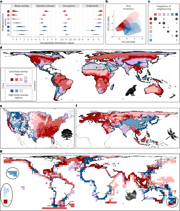
We identified geographical areas in biogeographical regions that exhibited similar biodiversity values, calling them biogeographical sectors. To characterize these biogeographical sectors, we used four biodiversity aspects that captured how biogeographical regions are the result of processes acting on both characteristic and non-characteristic species. These four biodiversity aspects were: the relative richness of characteristic species, which quantified how well a grid cell represented the characteristic species pool of a biogeographical region compared to other grid cells; the overlap of biotas, which measured the proportion of non-characteristic species in a grid cell; the relative occupancy of characteristic species, which measured the extent to which a characteristic species occupied its biogeographical region in comparison to other characteristic species of its biogeographical region; and the endemicity of characteristic species, which indicated the proportion of a characteristic species’ distribution range outside of its associated biogeographical region.

To quantify these four biodiversity aspects, we employed network cartography67, a widely used approach in multiple fields of science used for gaining insights into the organization and connectivity of elements in complex systems (in our case, species and grid cells). Specifically, we used two measures: the within-module degree (z) and the connectivity across modules (C) for both grid cells and species. These metrics informed us on the link distribution of nodes inside and outside their respective module67 (Extended Data Fig. 1). The z measures represented the relative connectivity of a given node within its associated module, measured as a z score ranging from minus infinity to infinity. For a grid cell, zcell indicated the relative species richness of the characteristic species in a grid cell compared to other grid cells in the same biogeographical region. In each module, the grid cell with the highest zcell best represented the characteristic species richness, and vice versa. For the species, zspp denoted the relative occupancy of a species in its associated biogeographical region compared to the other characteristic species. In each module, the characteristic species with the highest zspp occupied the largest area of the biogeographical region, and vice versa. Contrastingly, the connectivity across modules (C) measures the proportion of links of a node outside its module, ranging from 0 to 1. For the grid cells, Ccell measures the overlap of biotas as the proportion of non-characteristic species present in a given grid cell. Values of 0 indicate the absence of non-characteristic species with zero overlap of biotas, with lower values indicating the overlap of biotas. For example, a value of 0.4 would indicate that 40% of the species present in the grid cell were non-characteristic. For the species, Cspp measures the endemicity, quantified as the proportion of the characteristic species’ distribution area that fell within its biogeographical region. A value of 1 indicates that the characteristic species is endemic, with lower values indicating that part of its distributional area is also present in other biogeographical regions. To assign a value of occupancy, zspp, and endemicity, Cspp, to each grid cell, we selected their present characteristic species and calculated the median values of zzpp and Cspp (Extended Data Fig. 1). To quantify the four biodiversity aspects per grid cell, we defined:

$${\mathrm{Relative}}\,{\mathrm{species}}\,{\mathrm{richness}}=({I}_{c}-{\bar{I}}_{{m}_{c}})/{\sigma }_{{I}_{{m}_{c}}}$$

(1)

where Ic is the number of links of grid cell c to the species in its module, m, and \({\bar{I}}_{{m}_{c}}\) and \({\sigma }_{{I}_{{m}_{c}}}\) are the mean value and the standard deviation, respectively, of Ic over all grid cells in module m.

$${{\mathrm{Biota}}\; {\mathrm{overlap}}}={O}_{c}/{L}_{c},$$

(2)

where Oc is the number of links of grid cell c connecting with species outside its module, and Lc is the total number of links of grid cell c, including links inside (Ic) and outside (Oc) its module.

$${{\mathrm{Endemicity}}}={{\mathrm{Mdn}}}\left(\frac{{I}_{s}}{{L}_{s}}\right)\,,$$

(3)

where Is is the number of links of the present characteristic species, s, connecting with grid cells inside its module, and Ls is the total number of links of the present characteristic species, s, including links inside and outside its module, and Mdn is the median of the values of the present characteristic species in the grid cell.

$${{\mathrm{Relative}}\; {\mathrm{occupancy}}}={{\mathrm{Mdn}}}\left(\frac{{I}_{s}-\,{\bar{I}}_{{m}_{s}}}{{\sigma }_{{I}_{{m}_{s}}}}\right),$$

(4)

where \({\bar{I}}_{{m}_{s}}\) and \({\sigma }_{{I}_{{m}_{s}}}\) are the mean value and the standard deviation, respectively, of Is over all characteristic species in module m. We calculated the four biodiversity metrics in all the grid cells of each of the seven grids associated with the seven taxa.

The four biodiversity aspects did not strongly correlate (|Pearson’s coefficient| 68)), and provided complementary information (see correlation values for each taxon and overall in Supplementary Tables 1–8).

To divide the grid cells into biogeographical sectors, we followed a two-step approach. In the first step, we conducted the following procedure seven times, once per taxon. We selected the grid cells of a given taxon and performed a k-means analysis to identify clusters of geographical areas with similar combinations of the four biodiversity aspects. To determine the optimal number of clusters, for each taxon, we used an elbow-like69 method commonly employed in biogeography25,70. We tested cluster numbers ranging from two to 30, and calculated the goodness-of-fit (GoF), defined as the ratio of the between-cluster variance to the total variance. Recognizing the heuristic nature of k-means, we repeated each k-means clustering 100 times and selected the partition with the highest GoF in each partition with cluster numbers ranging from two to 30. Then, in a piecewise regression, we modelled the best 29 GoF values (dependent variable) with the number of clusters (explanatory variable) to identify the inflection point or point of sharpest decrease71, by searching for the cluster count that resulted in the lowest residual standard error. This point reflects where adding more clusters no longer substantially increases the GoF, and thus represents an optimal balance between model complexity and clustering quality. We identified this point using a brute force iterative search72. At this stage, we obtained seven outcomes, one per taxon, indicating the optimal partition of grid cells to taxon-specific biogeographical sectors (Supplementary Table 12). We used these outcomes in the second step.

In the second step, to address whether the biogeographical sectors were taxon-specific or general across the taxa, we performed a general k-means clustering analysis that included all 48,870 grid cells from the seven taxa jointly. We evaluated 13 potential partitions, ranging from two to 14 clusters, with the maximum number constrained by the results from the taxon-specific analyses (first step) and computational feasibility. These clusters, representing geographical areas with similar biodiversity characteristics across all taxa, were termed general biogeographical sectors. To determine the optimal number of clusters, we sought the partition in the general k-means that showed the highest similarity to the taxon-specific results. For each of the 13 potential partitions conducted with all grid cells from the seven taxa (2–14 clusters), we separated the grid cells of each taxon to create seven individual sets. For each partition and set, we quantified the similarity in grid-cell grouping between the general k-means (second step) and the taxon-specific k-means (first step) using adjusted mutual information (AMI), a widely accepted metric for assessing clustering similarity73. For each partition, we obtained seven AMI values, one per taxon, which were averaged to provide an overall similarity measure per partition. Our results showed that the partition with seven clusters produced the highest average AMI value. We considered that the seven-cluster partition provided the best description of biodiversity organization across the seven taxa, and used that as the basis for our subsequent analyses. Nevertheless, all subsequent results remained consistent, regardless of the number of clusters (sensitivity analyses using cluster 2–8 counts) (Supplementary Figs. 8–13 and Supplementary Tables 10 and 11). Although we chose the number of clusters that best represented all taxa, on average, the grid cells were free to group based on their biodiversity aspects. If the combinations of biodiversity aspects in the grid cells differed between taxa, the grid cells of each taxon were expected to form separate clusters. Conversely, if the combinations of biodiversity aspects were similar across taxa, the clusters would contain grid cells from all taxa.

All k-means clustering analyses, both taxon-specific and general, used the four biodiversity aspects of species richness, biota overlap, occupancy and endemicity as features. Before clustering, these metrics were standardized to account for different value ranges. We excluded those modules with missing values in any of the four metrics, including modules consisting solely of species without a clear biogeographical affinity, modules in which all the grid cells exhibited identical species richness and modules where all the species occupied an identical number of grid cells. These modules represented tiny biogeographical regions with non-biogeographical relevance to our goals.

Sensitivity analyses accounting for the distinct number of grid cells per taxon in the k-means clustering provided similar results (Extended Data Figs. 2–8, Supplementary Figs. 27–34 and details in Supplementary Information Appendix C). To maintain consistency in the k-means analyses in both the main and sensitivity analyses, we used the function kmeans.weight from the R package SWKM74 in both cases (Supplementary Information Appendix C). Additionally, sensitivity analyses accounting for the distinct geographical extent of the data (global and continental) when delineating the biogeographical regions and calculating the biodiversity metrics also provided similar results (Supplementary Information Appendix D).

In the Supplementary Material, we provide R code for estimating the four biodiversity aspects of biota overlap, species richness, species occupancy and species endemism. This code also enables the clustering of grid cells based on these aspects to identify biogeographical sectors. Furthermore, the online tool Infomap Bioregions, for mapping biogeographical regions54,61, now provides the values of these four biodiversity aspects (www.mapequation.org/bioregions2/).

Neighbour analyses

To examine the spatial relationship among biogeographical sectors, we assessed whether these sectors exhibited a higher degree of neighbourhood or adjacency to other sectors than expected by chance. With seven sectors, the expected chance probability of neighbouring a different sector was 1 in 6. To calculate the observed probability, we identified neighbouring grid cells belonging to different biogeographical sectors. Then, we evaluated whether the observed neighbouring probability surpassed the expected chance probability through binomial proportional tests. To account for variations in the number of neighbouring grid cells across different biogeographical sectors, we performed tests in both directions, assessing the neighbourhood between hypothetical sectors A and B (A → B and B → A). We deemed there was evidence of significant neighbourhood if either the A → B or B → A tests yielded P 75. The results are illustrated in Fig. 1c, where the circle sizes represent the relative proportion of statistically significant neighbouring events across sector pairs in all biogeographical regions and taxa. Supplementary Table 9 provides details on the total number of biogeographical regions, across the seven taxa, where the two compared biogeographical sectors were represented—that is, at least one grid cell from each of the two sectors. Supplementary Table 9 provides details on the proportion of those latter regions where neighbouring between pairs of sectors was higher than expected.

Multinomial models

We examined whether the biogeographical sectors corresponded to geographical areas with distinct environmental conditions by using multinomial logit models with biogeographical sectors as the response variable. We assessed the existence of a correlation between the core-to-transition pattern with two widely used variables for explaining species diversity at the global scale: mean annual temperature and precipitation for the terrestrial biota and mean surface temperature and salinity for the marine biota. The data on mean annual temperature and precipitation were obtained from the Climatic Research Unit time series dataset v.4.06 (ref. 76) and downscaled using WorldClim v.2.1 (ref. 77), with the mean sea-surface temperature and sea-surface salinity data being obtained from the National Aeronautics and Space Administration’s Ocean Color Web website (http://oceancolor.gsfc.nasa.gov/) and the National Oceanic and Atmospheric Administration’s World Ocean Atlas 2009, and prepared by Sbrocco and Barber78. To align the raster data with our grid, we computed the mean values of corresponding pixels within each grid cell.

We performed multinomial models for each taxon and biogeographical region, comparing a model including the two respective explanatory variables against a null model including only an intercept. Evidence was considered statistically significant if the difference in the corrected Akaike information criterion value exceeded 10 (ref. 79). We analysed biogeographical regions with two or more sectors. To mitigate issues with sample size in multinomial models, we only evaluated biogeographical sectors with more than 15 grid cells. To ensure the representativeness of the complete biogeographical region, we only evaluated those biogeographical regions where the sum of the biogeographical sectors with more than 15 grid cells represented at least 90% of the entire region. To assess the fit of the multinomial models, we used McFadden’s pseudo-R2. We performed multinomial models using the multinom function from the R package nnet80, and we calculated McFadden’s R2 using the PseudoR2 function from the R package DescTools81.

We also explored the potential correlation between present biodiversity and past climatic conditions (Supplementary Information Appendix A). We conducted sensitivity analyses to consider the spatial autocorrelation in the model residuals, obtaining similar results (Supplementary Information Appendix E).

Taxonomic dissimilarity: nestedness versus turnover

We examined whether the variation in species composition among biogeographical sectors, measured by Sørensen pairwise dissimilarity, was more attributed to nestedness or to species turnover components38. In our case, nestedness refers to dissimilarity arising because the species composition in one biogeographical sector is a subset of the species found in another sector, whereas turnover captures dissimilarity due to species replacement38. For each bioregion and taxon, considering all present biogeographical sectors together, we computed the proportion of the taxonomic dissimilarity between sectors attributed to nestedness. This proportion was calculated as the ratio of the nestedness component to the total Sørensen dissimilarity. We calculated the distinct components using the beta.multi function from the R package betapart82. We calculated the nestedness for characteristic and non-characteristic species separately. Because the non-characteristic species can be affined to distinct biogeographical regions, we conducted independent analyses for the non-characteristic species affiliated with each biogeographical region.

Local variation in species richness at the global scale

At our grid-cell resolution, variations in species richness were expected to depend on both the size of the regional species pool—resulting from the balance of speciation, extinction and biogeographical dispersal45,46—and the sorting of species from that pool47,48—in this study, associated with the core-to-transition organization and environmental filters. Previous studies has approximated the size of the regional species pool as the average species richness across locations within a biogeographical region46. Thus, the centred richness, calculated as the observed species richness in each grid cell minus the average richness in that biogeographical region, may be considered as representing species sorting within the region independently of the pool size. Therefore, to assess the relative importance of these factors, we modelled species richness across grid cells using three explanatory variables: (1) the total number of characteristic species per biogeographical region, obtained from the network analyses (a proxy for the size of the regional species pool); (2) the centred richness of characteristic species; and (3) the centred richness of non-characteristic species. These three variables provide an approximate decomposition of species richness. While these three variables together should explain a large proportion of the variance in species richness, this decomposition allowed us to explore the independent effect of each variable, and thus which regional effect was more relevant in explaining the global variance in local species richness. The size of the regional species pool would be more important in explaining global patterns in species richness if there were large differences in the size of the regional species pool among the biogeographic regions and the core-to-transition organization was, in general, driven by relatively few species. By contrast, the sorting of characteristic and non-characteristic species would be more important if there were small variations in the size of the regional species pools, and the core-to-transition organization was driven by relatively many species. These alternatives informed on whether global variations in species richness are more associated with the formation of the biogeographical regions and the species diversification and dispersals (size of regional species pool) or with the sorting of species due to environmental filters (core-to-transition organization).

To evaluate the relative importance of each factor, we fitted linear models of the grid-cell richness as a function of the three aforementioned variables. Then, we calculated the variance partitioning of the three explanatory variables, focusing on the individual fraction explained by those—that is, the variance explained by a variable after removing the variance shared with the other explanatory variables. This individual fraction of variance of a given variable was measured as the difference between the R2 of the saturated model and the R2 of a model without the focal variable. To prevent inference biases stemming from larger biogeographical regions, we used weighted regression, where the cell values were weighted by the inverse size of the biogeographical region. The results from this sensitivity analysis were qualitatively similar using unweighted regression (Supplementary Fig. 35). We performed linear regressions using the lm function from the R package stats75, and obtained the adjusted R2 by applying the R function summary to the output of the linear regression models.

Species richness in core area higher than expected

The core areas of each biogeographical region tend to comprise 30% of the biogeographical region while harbouring more species than the remaining 70%. This observation suggests a potential conservation value for these core areas50. To assess whether the species richness was higher than expected by chance, we conducted a randomization test for each combination of biogeographical region and taxon. We randomized the identity of the biogeographical sectors in the grid cells while maintaining the total number of grid cells per biogeographical sector and region. This process was repeated 100 times. We then evaluated whether the observed species richness in the core areas was higher than that in the randomized core.

Reporting summary

Further information on research design is available in the Nature Portfolio Reporting Summary linked to this article.