Development of scMicro-C
The previously reported bulk Micro-C chemistry, although offering nucleosome-level contact maps, cannot be applied to single cells because of substantial loss of DNA caused by overdigestion and low ligation efficiency34,35. To achieve scMicro-C, we implemented three key improvements (Fig. 1a; Methods). First, we employed an ionic detergent (sodium dodecyl sulfate (SDS)) to solubilize chromatin and improve ligation efficiency. Second, we systematically titrated the degree of MNase digestion to assess the effect on chromatin structure detection. Third, we omitted biotin enrichment and adopted a transposon-based whole-genome amplification (WGA) technique called multiplex end-tagging amplification (META)37 to enhance the detection of chromatin contacts.
Fig. 1: Development of scMicro-C.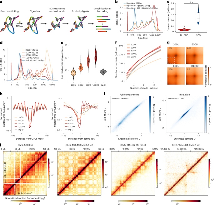
a, Schematic of the scMicro-C procedure. b, Chromatin length distribution to compare the ligation efficiency between SDS treatment and the original Micro-C protocol. Data generated by the capillary electrogram. c, Violin plot to compare the contact number between SDS treatment and original protocol (SDS, n = 22; original, n = 33). The box middle line represents the median value, the box limits the 25% and 75% quantiles, and the whiskers show the minimum and maximum. d, The chromatin length distribution depicts the degree of digestion resulting from MNase titration. e,f, Comparison among scMicro-C with different MNase titration and Dip-C, showing the percentage of reads containing contacts (e); the horizontal line and the box represent the median and quartiles, respectively (bottom). The whiskers indicate minima and maxima (e) and a downsample plot depicting the relationship between the number of reads and the number of unique contacts (f). The line indicates the median value, and the shadow indicates the 95% confidence interval. (f). 200U, n = 96; 600U, n = 96; 800U, n = 96; 1,000U, n = 96 and Dip-C, n = 17. g, Pile-up results of chromatin loops (bulk Micro-C detected loop set, n = 45,174) for four MNase titration groups. h, Normalized nucleosome occupancy around CTCF binding sites (left) and active TSS (right) of five scMicro-C datasets. i, Two-dimensional histograms to show the correlation of A/B compartment values at 100-kb resolution (left) and insulation scores at 10-kb resolution (right) between ensemble scMicro-C and bulk Micro-C. j, Contact maps of ensemble scMicro-C (top left) and bulk Micro-C (bottom right) at 500 kb, 50 kb, 5 kb and 1 kb from left to right to show the compartments, TADs and chromatin loops, respectively. TADs, topologically associating domains.
Inspired by the Hi-C procedure38, we introduced SDS treatment after MNase fragmentation in the Micro-C procedure. This step improved the chromatin accessibility for end-repair enzymes, thereby boosting ligation efficiency compared to the original bulk Micro-C procedure34,35, independent of chromatin digestion levels (Fig. 1b and Extended Data Fig. 1a). To test whether enhanced ligation efficiency improves the detection of chromatin contacts in individual cells, we isolated and processed single cells and performed WGA and sequencing. The data show that SDS treatment increases detected chromatin contacts by 8.1 times at similar sequencing depths (Fig. 1c, Extended Data Fig. 1b–d and Supplementary Table 1). This may be attributable to the larger size of end repair enzymes (T4 polynucleotide kinase = 132 kDa and Klenow fragment = 68.2 kDa) compared to MNase (16.9 kDa), which poses challenges in accessing chromatin without SDS.
After establishing a protocol with high ligation efficiency, we next aimed to investigate how MNase digestion levels impact chromatin structure detection in scMicro-C experiments. Using four distinct MNase concentrations (200U, 600U, 800U and 1,000U containing approximately 4 million nuclei in a 100-μl reaction volume), we tested varying digestion degrees from low to high (Fig. 1d). Notably, even the highest concentration (1,000U) did not reach the level of digestion of standard bulk Micro-C. We note that the high degree of digestion in bulk Micro-C statistically diminished ligation efficiency (Extended Data Fig. 1a), as previously observed in the Micro-Capture-C (MCC) procedure39. Subsequently, we employed fluorescence-activated nuclei sorting to sort individual nuclei into a 96-well plate for each MNase concentration. Sequencing analysis revealed median counts of chromatin contacts per cell—671.6k (200U), 817.1k (600U), 863.2k (800U) and 874.4k (1,000U; Extended Data Fig. 2a). We observed slightly increased inter-chromosomal contacts at higher levels of MNase digestion (Extended Data Fig. 2b).
With increasing MNase concentration, the single-cell profiles exhibited a higher percentage of reads containing contacts (referred to as contact ratio) and a greater number of unique contacts at the same sequencing depth (Fig. 1e,f and Extended Data Fig. 2c). We note that the contact ratio is compromised when compared to bulk Micro-C employing biotin pulldown, but is notably higher than our previously developed scHi-C method, Dip-C37, particularly at higher MNase concentrations (Fig. 1e,f).
Notably, we found that chromatin structures across various scales remain largely consistent among different MNase concentrations (Fig. 1g and Extended Data Fig. 2d–g). Like bulk Micro-C, scMicro-C preserves nucleosome occupancy and TF footprinting profiles39, with nucleosome occupancy profiles becoming slightly sharper at higher MNase concentrations (Fig. 1h and Extended Data Fig. 3). These features are not offered by restriction enzyme-based scHi-C (Fig. 1h and Extended Data Fig. 3). Based on our observations, we determined that the optimal choice for scMicro-C experiments is a digestion level of 800U.
Following the optimal scMicro-C procedure, we applied scMicro-C to GM12878 cells. In total, we profiled over 800 GM12878 cells (Supplementary Table 1) and kept 724 high-quality cells after quality control (Methods), achieving a median of 835k unique chromatin contacts per cell (s.d. = 467k, min = 228k and max = 3.5 m). To assess the fidelity of scMicro-C in capturing multiscale 3D genome organization, we aggregated all single-cell profiles (referred to as ensemble scMicro-C), yielding a contact map containing 750 million contacts.
To validate our modified Micro-C methodology, we generated two bulk Micro-C datasets for GM12878 cells using distinct protocols, as detailed in the Methods (modified bulk Micro-C). One dataset adhered to our modified Micro-C protocol, denoted as dataset 1, while the other dataset was produced using the original Micro-C procedure34, designated as dataset 2. The comparison between the two datasets confirms that the modified protocol does not compromise data quality (Supplementary Fig. 1). Together, the two datasets yielded a total of 4.4 billion valid contacts. Upon comparison with published GM12878 Hi-C data at the highest available sequencing depth (4.9 billion contacts)40, our bulk Micro-C data exhibited a higher signal-to-noise ratio, as evidenced by a greater number of chromatin loops (HICCUPS—20882 versus 9738) and chromatin stripes (Stripenn—3414 versus 2722), and stronger chromatin loop and stripe signals (Supplementary Fig. 2).
Comparison between bulk Micro-C and ensemble scMicro-C reveals a high level of agreement across scales, encompassing A/B compartments, topologically associating domains and fine-scale chromatin loops (Fig. 1i,j). Notably, ensemble scMicro-C delineates chromatin features at resolutions as fine as 1 kb (Extended Data Fig. 4c). Quantitatively, our bulk Micro-C achieves 1-kb resolution, and ensemble scMicro-C 5-kb resolution (Supplementary Fig. 3; Methods), with resolution defined as previously described40. Additionally, akin to Micro-C, when compared to bulk Hi-C and scHi-C methodologies, scMicro-C exhibits a superior signal-to-noise ratio in the detection of chromatin loops and stripes (Extended Data Fig. 4).
scMicro-C resolves 3D genomes at kilobase resolution
Contact map-based analysis is inherently limited to two dimensions and is unable to accurately determine the position of genomic loci in 3D space. To address this limitation, several algorithms have been devised for reconstructing the 3D genome structure of both haploid and diploid cells from single-cell contact maps37,41,42, providing insights into the radial organization of genomic loci43, chromosome compaction37 and multiway interactions. Notably, our previous restriction enzyme-based Dip-C method enabled the reconstruction of 3D genome structures of diploid cells at 20-kb resolution37. A resolution of 20 kb signifies that each particle of the 3D genome structure reconstruction represents a genomic locus of 20 kb. The definition of resolution is data-driven, reflecting minimal variability across multiple independent reconstructions (Methods). This concept aligns with DNA FISH-based microscopy methods. Despite this advancement, the 20-kb resolution of the current scHi-C technique remains insufficient for investigating the intricate folding patterns of finer-scale structures like E–P loops and chromatin stripes.
Applying our previously developed Dip-C algorithm to scMicro-C data, we reconstructed 3D genome structures of individual GM12878 cells (Methods). Among the 724 cells analyzed, 358 cells (49.4%), 335 cells (46.1%) and 281 cells (38.8%) resolve whole-cell 3D genome structures of 20-kb, 10-kb and 5-kb resolution, respectively. Only cells demonstrating low uncertainty at each specific resolution were considered for downstream structure-based analysis (Methods). Quality control confirmed that cells displayed high consistency across different replicates and resolutions (Extended Data Fig. 5a,b). The attainment of 3D genome structures at a 5-kb ‘particle size’ enables the exploration of the finer-scale folding intricacies within chromatin structures (Fig. 2a).
Fig. 2: Kilobase 3D genome structures of scMicro-C.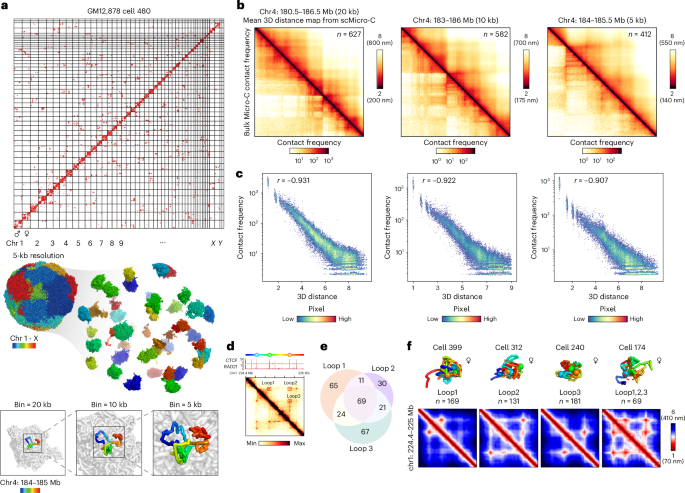
a, A haplotype-imputed contact map of a representative GM12878 cell (top), the corresponding reconstructed 3D genome structure at 5-kb resolution (middle) and a selected region (chr4: 184–185 Mb) are shown at 20-kb, 10-kb and 5-kb resolution (bottom). b, Heatmaps show the mean 3D distance matrices measured from single-cell 3D genome structures (top right) and the bulk contact frequency maps (bottom left) for the corresponding regions at 20-kb, 10-kb and 5-kb resolution, respectively. c, Scatter plots show the correlation between mean 3D distance measured from single-cell 3D genome structures and contact probability measured from bulk Micro-C at 20-kb, 10-kb and 5-kb resolution, respectively, of the same region at b. d, Contact map of a nested chromatin loop region (chr1: 224.4–225 Mb), CTCF and RAD21 ChIP–seq tracks, and cartoon schematics of three loop anchors were shown at the top. e, Venn diagram to show the overlap of the occurrence of three nested chromatin loops. A chromatin loop was defined as being formed when the 3D distance between two loop anchors was less than 3.5 particle radii (~240 nm). For this region, 428 single-cell 3D structures were available. The co-occurrence between loop1 and loop2, P = 2.3 × 10⁻⁹; co-occurrence between loop1 and loop3, P = 2.43 × 10⁻⁵; co-occurrence between loop1 and loop3, P = 1.02 × 10⁻¹². A hypergeometric test (one-sided) was used. f, Representative single-cell 3D chromatin structures (top) and corresponding mean 3D distance matrices (bottom) for forming loop1, loop2, loop3 and co-occurrence of three loops.
To assess the fidelity of the reconstructed single-cell 3D genome structures, we measured the pairwise 3D distance matrices, which exhibit a high degree of anticorrelation with bulk Micro-C contact frequency across various resolutions (Pearson’s r values = −0.931 at 20 kb, −0.922 at 10 kb and −0.907 at 5 kb; Fig. 2b,c). Consistent results were also observed in other genomic regions (Extended Data Fig. 5c). These findings confirmed that the single-cell kilobase-resolution 3D structures resolved by scMicro-C are both reliable and rich in information.
Reanalysis of deeply sequenced Dip-C data revealed the presence of limited 5-kb resolution cells. Despite the limited number of Dip-C cells, we compared the reconstructed 3D genome structures with those obtained from scMicro-C and observed a high level of consistency between the two methods (Extended Data Fig. 5d,e). However, the low number of 5-kb resolution Dip-C cells precludes quantitative benchmarking. Nonetheless, based on the visual comparison of contact maps, we speculate that scMicro-C-derived 3D genome structures offer superior analysis of fine-scale chromatin structure compared to restriction enzyme-based Dip-C.
Using hundreds of 5-kb single-cell 3D genome structures, we investigated fine-scale chromatin folding, particularly multiway interactions. Although the majority of contacts identified through scMicro-C were pairwise, multiple pairwise interactions within a 5-kb bin implied simultaneous multi-loci proximity in 3D genome structures. Focusing on the nested CTCF-anchored chromatin loop (Fig. 2d), characterized by the formation of pairwise chromatin loops between loop anchors, we assessed whether these formed independently or concurrently (Supplementary Fig. 4a). Analysis of the overlaps in single-cell 3D structures that form these loops revealed a statistically significant tendency for nested chromatin loops to form simultaneously (Fig. 2e). Our scMicro-C 3D structures directly visualized the dynamic loop formation events (Fig. 2f and Supplementary Fig. 4b), with similar results observed in other regions featuring nested chromatin loops (Supplementary Fig. 4c–h). Nested chromatin loop formation was also observed in the SPRITE and MC-4C techniques12,17, which detect multi-way high-order interactions. We speculate that the concurrence of nested CTCF loops is driven by the synergistic stabilization effect of spatially clustered CTCFs, which protects cohesin against WAPL-mediated release44.
Characterization of promoter–enhancer stripe (PES)
We next focused on analyzing E–P interactions. We observed that a large number of genes displayed a distinct PES chromatin structure, characterized by a line-like structure on the chromatin contact map. These stripes are anchored at the transcription start site (TSS) and extend in the direction of transcription, indicating frequent and sustained promoter–gene body interactions (Extended Data Fig. 6a).
A similar stripe structure has been reported in previous studies, including at the SOX9 gene (referred to as a promoter-associated stripe), in the Hi-C pile-up analysis of Stag2-knockout-downregulated genes (referred to as promoter-anchored stripes) and in the pile-up results at the active promoter region of bulk Micro-C data (referred to as gene stripes)34,45,46, albeit with a limited number of genes and without extensive characterization. Here we named genes exhibiting this PES configuration as ‘PES genes’, which included key TFs essential for B-cell function, such as early B cell factor 1 (EBF1) and interferon regulatory factor 2 (IRF2). In contrast to PES, previous studies focused primarily on ‘architectural stripes’, which are commonly located at topologically associating domain boundaries and formed between two strong convergently oriented CTCF binding sites47. These architectural stripes are typically longer and stronger than PES (Supplementary Fig. 1f) and are not always associated with genes. However, it remains possible that certain PES overlap with or could themselves be considered architectural stripes.
Upon examination, we observed the presence of multiple H3K27ac-marked enhancers distributed along the PES (Extended Data Fig. 6a). Noticeably, these stripes frequently exhibited focal interactions at the enhancer sites (Extended Data Fig. 6a). Motivated by this observation, we performed de novo detection of PES genes in GM12878 using our bulk Micro-C dataset. We identified 819 genes with PES of 4,077 active long genes (≥50 kb) in GM12878, and pile-up results confirmed the existence of the PES (Fig. 3a and Extended Data Fig. 6b,c). Notably, genes with PES exhibit significantly higher expression levels than genes without (P = 9.88 × 10⁻⁹; Fig. 3b).
Fig. 3: Characterization of PESs.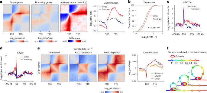
a, Pile-up results of GM12878 PES genes (left, n = 819), length-distribution-matched non-PES genes (left center, n = 819) and the difference between stripy and nonstripy genes at 1-kb resolution (right center). Right, pile-up results, rescaled between the TSS and the TTS. b, Cumulative curves of expression level for PES and non-PES genes of GM12878. A two-sided Mann–Whitney U test was used. c, Metagene plots of mean H3K27ac signal of stripy and nonstripy genes of GM12878. d, Metagene plots of mean RAD21 signal of PES and non-PES genes of GM12878. e, Pile-up results of PES genes (n = 853) for untreated, RAD21-depleted and WAPL-depleted Micro-C data from mESC at 1-kb resolution. Signal value along the TSS is shown on the far right. Data are from ref. 49. f, Cartoon model depicting cohesin-mediated loop extrusion facilitating the scanning of downstream enhancers by the promoter.
Metagene analysis revealed stronger enhancer signals (as indicated by the H3K27ac signal) in stripy and nonstripy gene bodies (Fig. 3c). These findings were reinforced by activity-by-contact model predictions48, which identified multiple stripy gene-associated enhancers distributed along PES (Extended Data Fig. 7a–c,i). Promoter–enhancer interaction pile-ups revealed localized intensity peaks at enhancer loci (Extended Data Fig. 6d), and robust interactions among multiple enhancers regulating the same stripy gene suggested the formation of enhancer hubs (Extended Data Fig. 6e). Collectively, these findings suggest that the potential function of the PES is to facilitate interactions between the promoter and multiple downstream enhancers.
We then focused on elucidating the mechanism of PES formation. We noted statistically stronger cohesin binding at stripy gene promoters compared to nonstripy genes, as indicated by cohesin subunits RAD21, SMC1A and SMC3 (Fig. 3d and Extended Data Fig. 7f,i), indicating cohesin’s involvement in PES establishment. To test this hypothesis, we examined the effects of cohesin depletion using a Micro-C dataset in mouse embryonic stem cells (mESC)49 and observed statistically reduced PES formation after cohesin depletion. While cohesin unloading factor—WAPL depletion extended PES downstream (Fig. 3e and Extended Data Fig. 7g,h). These experiments demonstrate that PES formation is dependent on cohesin-mediated loop extrusion.
We next investigated whether E–P and enhancer–enhancer (E–E) interactions in genes with PES were influenced by the depletion of cohesin. Our re-analysis of this cohesin depletion Micro-C data49 in the context of PES confirms that both E–P and E–E interactions were statistically attenuated following cohesin depletion, with a more pronounced reduction in stripy compared to nonstripy genes (Extended Data Fig. 7j,k). Specifically, 21% of E–P interactions in genes with PES were identified as E–P loops, compared to 10.5% in genes without PES. Among these E–P loops, 48.5% in PES genes were statistically weakened, whereas only 35.5% of E–P loops in genes without PES exhibited such weakening (Extended Data Fig. 7l).
Given the data, we hypothesize that cohesin-mediated loop extrusion facilitates promoter scanning of downstream genomic loci, thereby fostering interactions with multiple enhancers (Fig. 3f). However, further mechanistic studies are required to test this hypothesis. Intriguingly, the presence of nested tiny stripes derived from enhancers in certain stripy genes indicates that the scanning may also be initiated from enhancers (Extended Data Fig. 6a), a possibility that is not represented in the current model schematic.
scMicro-C visualizes dynamic E–P interactions in PES genes
Upon gaining an understanding of the function and formation mechanism of PES, we aimed to characterize the E–P interactions of genes with PES. To do this, we used scMicro-C data to visualize the 3D structure of a specific PES gene called EBF1. This gene is located on chromosome 5, spans 404 kb, and has an expression level of 7.59 FPKM. EBF1 is a key regulator of B cell lineage development50.
The EBF1 locus exhibits a distinct PES on the bulk Micro-C and ensemble scMicro-C contact map, connecting its promoter to seven activity-by-contact model-predicted EBF1 enhancers (named E1–E7; Fig. 4a). Notably, multiple nested weak stripes within the EBF1 PES connecting multiple enhancers were clearly visible (Fig. 4a).
Fig. 4: Multi-enhancer hubs captured by single-cell high-resolution 3D genome structures.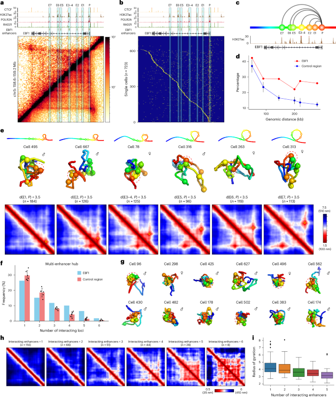
a, Contact map of ensemble scMicro-C (top left) and bulk Micro-C (bottom right) at the EBF1 locus, accompanied by ChIP-seq signals of CTCF, H3K27ac, POLR2A and RAD21, and ABC model-predicted enhancers. b, Sorted scMicro-C contact profiles (n = 723) of the EBF1 gene with PES; the 5-kb bins covering the EBF1 TSS were used for this analysis. c, Schematic representation of the promoter and enhancers of the EBF1 gene selected for single-cell 3D genome structure analysis. d, Line plot showing the percentage of single-cell 3D chromatin structures with the proximity of corresponding E–P pairs. Six regions without stripes were used as controls. The dots indicate the median value, and the whiskers of control regions indicate the standard deviation. e, Top row, schematic representation of the E–P loops in each cell (columns). Middle row, representative single-cell 3D structure of the E–P loops. Bottom row, mean 3D distance matrices of single-cell structures, with the depicted loop indicated by a yellow circle. f, Bar plot of the percentage of cells (y axis) that have the indicated number of enhancer interactions with the promoter (x axis) at the EBF1 (blue) or control locus (red). For the EBF1 locus, the number of cells is indicated at the top of each bar. For control regions, the bar indicates the median value, and the error bar indicates the s.d. g, Representative single-cell 3D genome structures forming a multi-enhancer hub (red dashed circles) at EBF1. h, Mean 3D distance matrices measured from single-cell structures with the indicated number of enhancer loci interacting with EBF1 promoter from left to right, respectively. i, Boxplot of the radius of gyration (y-axis) of single-cell 3D genome structures with the indicated number of enhancer loci (x axis—n = 114, n = 66, n = 51, n = 44, n = 28, n = 8 for each group) interacting with the EBF1 promoter. Pairwise statistical tests showed statistical significance (P
To explore the dynamics of PES formation, we sorted single-cell contact maps based on interactions with the TSS region, observing a gradual transition of contacts from the TSS to downstream regions (Fig. 4b). This series of snapshots captures the dynamic contact between the TSS and downstream loci, highlighting the dynamic nature of the observed ‘stripes’ across individual cells. In addition to the main transition line, sporadic contacts were also noted, indicating multiple pairwise interactions between downstream loci and the TSS in individual cells (Fig. 4b).
Three-dimensional distance analysis of six enhancer loci (E1–E7, E3/E4 merged at 5-kb resolution; Fig. 4c) showed looping events between EBF1 promoter and downstream enhancers (E2–E7) occurring in approximately 30% of single-cell structures (Fig. 4d), with a looping event defined as a 3D distance between the TSS (P) and another locus (E1–E7) less than 3.5 particle radii (~240 nm, see Methods). This frequency contrasts with nonstripy controls, where looping frequency declined with genomic distance (Fig. 4d and Supplementary Fig. 5), indicating that genes exhibiting PES have a higher frequency of E–P interactions.
We visualized the dynamic looping process of PES using single-cell 3D genome structures, directly capturing the dynamic E–P looping events between the promoter and multiple downstream enhancers (Fig. 4e). Our observations at the EBF1 locus were corroborated by similar findings in the analysis of the IRF2 gene (chr4: 88.9 kb, 47.7 FPKM), which, like EBF1 exhibited a prominent PES structure and contained multiple enhancers within the stripe region (Extended Data Fig. 8a–d). These findings collectively suggest that E–P interactions are highly dynamic and heterogeneous among individual cells. It is important to note that while our observations provide insights into the dynamics of looping events based on snapshots of single-cell 3D genome structures, live-imaging techniques are needed for direct visualization of these dynamic chromatin looping events51,52.
Multi-enhancer hubs observed in single-cell 3D genomes
How multiple enhancers are spatially organized to regulate gene expression is not extensively studied. Previous studies using long-read 3C derivatives revealed cooperative 3D interactions between regulatory elements14,15, such as simultaneous interactions between multiple enhancers and promoters at the α/β-globin gene locus12,53 and interchromosomal multi-enhancer hubs regulating olfactory receptors (ORs)54.
We aimed to understand how the multiple enhancers of stripy genes are arranged within individual 3D structures. Upon analyzing single-cell 3D structures at the EBF1 locus, we observed a statistically significant number of structures in which more than one enhancer simultaneously interacts with the EBF1 promoter (Fig. 4f). We refer to this structure as a ‘multi-enhancer hub’. Three-dimensional visualization of these multi-enhancer hubs in individual cells revealed a spatial cluster of enhancers associating with the EBF1 promoter (Fig. 4g). The simultaneous interaction between the EBF1 promoter and multiple enhancers was also supported by findings from the scNanoHi-C study, which uses third-generation long-read sequencing to capture high-order multiway interactions14.
Further examination of the 3D distance matrix of single-cell structures harboring between one and six enhancers revealed that a higher number of enhancers in the hub led to a more extensive interconnected enhancer network (Fig. 4h). Additionally, we observed that with an increase in the number of enhancers, chromatin structure became more compacted, as indicated by a decrease in the radius of gyration (Fig. 4i). These results highlight the cooperative interactions between multiple enhancers in association with the promoter, suggesting a distinctive mechanism of enhancer regulation in stripy genes.
To ascertain whether the presence of multi-enhancer hubs is a common feature among stripy genes or specific to the EBF1 gene, we investigated several other stripy genes, including IRF2 and PIEZO2. Analysis revealed the existence of multi-enhancer hub structures in these genes as well (Extended Data Fig. 8f and Supplementary Fig. 6a–e). This prevalence of multi-enhancer hubs was signified by the extensive E–E interactions observed in stripy genes (Extended Data Fig. 6c), confirming the assembly of multi-enhancer hubs. Additionally, the conclusions regarding interenhancer connectivity and chromatin compaction were confirmed within the IRF2 gene locus (Extended Data Fig. 8g,h).
In conclusion, single-cell kilobase-resolution 3D genome structures generated through scMicro-C technology allow for the investigation of E–P interactions at the single-cell level. This approach has unveiled the dynamic and heterogeneous nature of E–P interactions within individual cells, leading to the identification of multi-enhancer hub structures in stripy genes. These findings offer valuable insights into the distinct regulatory mechanisms governing stripy genes through the coordination of multiple enhancers.
Polymer simulations of PES genes
To dissect the mechanisms driving multi-enhancer interaction networks in genes with PES, we conducted polymer simulations using the open2c ‘polychrom’ framework. We simulated the EBF1 locus with the following three key tunable parameters: cohesin-mediated loop extrusion (cohesin density, extrusion speed), cohesin capture probability of enhancers, and molecular affinities between promoters and enhancers (Extended Data Fig. 9a; Methods).
In our simulation settings, we positioned two strong boundary elements at the TSS and TTS of the EBF1 gene, reflecting CTCF binding at these sites (Extended Data Fig. 9a,b). Consistent with previous studies, cohesin blocking was sufficient to establish the stripe pattern46,47. However, in the absence of E–P/E–E molecular affinities and enhancer-mediated cohesin capture, neither apparent E–P/E–E loops nor enhancer stripes formed (Extended Data Fig. 9c, left). Introducing strong molecular affinities among enhancers and the promoter generates E–P/E–E interactions but fails to replicate stripes unless weak cohesin capture by enhancers was included (Extended Data Fig. 9c–e). These patterns completely disappeared upon cohesin depletion. Strong E–P and E–E affinities combined with cohesin capture by enhancers best match experimental observations (Extended Data Fig. 9d,e, right).
Because the above observations were derived from population-ensemble contact maps, we next focused on single chromatin fiber traces to verify the existence of multi-enhancer hub structures in these simulations. We found that only simulations with strong affinities among promoters and enhancers and cohesin capture by enhancers produced a prominent number of multi-enhancer hub structures (Extended Data Fig. 10a,b). The multi-enhancer hub structures were almost completely depleted in the absence of cohesin (Extended Data Fig. 10a,b). Additionally, the distance matrices from simulated structures closely resemble observations from scMicro-C 3D genome structures (Extended Data Fig. 10c,d).
In summary, computational modeling of 3D chromatin folding provides a complementary approach for exploring possible regulatory mechanisms underlying stripe gene folding, offering insights that are challenging to obtain experimentally. The simulations also confirm the physical feasibility of interconnected multi-enhancer networks at the single-chromatin fiber level.