MSnLib: efficient generation of open multi-stage fragmentation mass spectral libraries

Materials

All solvents used were of LC–MS grade. Methanol, acetonitrile, water and formic acid were obtained from Thermo Scientific. Seven different compound libraries, that were available to us, were analyzed: the NIH NPAC ACONN collection of natural products provided by the US National Institute of Health (NIH) with 3,988 compounds (NIHNP), a peptidomimetic library provided by OTAVAchemicals (Ontario, Canada) comprising 1,298 compounds (OTAVAPEP), the Discovery Diverse Set DDS-10 library from Enamine (Kyiv, Ukraine) with 10,240 compounds (ENAMDISC), a library mixture of 4,378 compounds purchased from Enamine and Molport (Riga, Latvia) including the 4,000 carboxylic acid fragment library (ENAMMOL), and three other libraries purchased from MedChemExpress (MCE, New Jersey, USA) containing 10,315 bioactive compounds (MCEBIO), 5,000 compounds from the MCE 5K Scaffold Library (MCESCAF), and 2,610 Food and Drug Administration-approved drugs (MCEDRUG). More information on compounds is given in Supplementary Note 1.

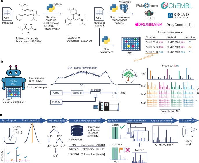
General workflow

1. 1.

   Metadata clean-up

   1. a.

      Manual harmonization of input metadata sheet and column names

   2. b.

      Defining jobs and running jobs.py

2. 2.

   Sequence generation

3. 3.

   Sample preparation (mixing compounds)

4. 4.

   Data acquisition

5. 5.

   Automatic MSn tree library creation and data evaluation in mzmine

   1. a.

      Combining the cleaned metadata with the acquired data

Metadata clean-up

A Python script (metadata_cleanup_prefect.py) was developed for the curation of metadata. The main purpose of this script is structure extraction, salt removal, and standardization. Structure standardization was based on the ChEMBL structure pipeline Python package18. The complete clean-up failed with the original pipeline for specific structures (when a salt was given without a dot in the structure) and required an additional initial salt removal step and a second clean-up run. The cleaned and standardized structure is used for calculating other structural information such as canonical and, if available, isomeric SMILES (simplified molecular input line entry system), InChI (international chemical identifier developed by the International Union of Pure and Applied Chemistry), InChIKey (a condensed version of InChI), logP (the logarithm of the octanol–water partition coefficient) and monoisotopic mass. This mass is used during the automatic library generation. Optionally, additional information, such as whether a compound is considered a natural product or used as a drug, can be gathered from other databases based on a name, database identifier or structure search in PubChem, ChEMBL or other public resources (Supplementary Note 2). Queries can be easily turned off or implemented in the Python code. In our code, all databases that require a local file are deactivated by default.

Sequence generation

An additional Python script (sequence_creation.py) was used to prepare the sequence table based on plate and well information. The sequence for each plate is built so that it is first analyzed in positive ion mode, followed by negative ionization. A file name is generated automatically and contains the date, a unique sample identifier (combination of library, plate number and well location), the method used, and the polarity. The unique sample identifier is important because it is used for the automatic annotation and extraction of the acquired spectral data. Therefore, the unique sample identifier in the metadata column needs to be matched with a substring of the acquisition file name. Here, only this identifier is important in the name, enabling the addition of other prefixes and suffixes, for example, the date, polarity or method. The script generates acquisition sequence files specific to the Xcalibur sequence layout using the flow injection–Orbitrap MSn method. This can be easily modified for other analysis platforms, depending on their layout.

Sample preparation

Our mass spectral library contains seven different compound libraries. The MCEBIO library was prepared with an OT-2 liquid handler (Opentrons Labwork) to pool and dilute 10 compounds in each well of three 384-well plates, resulting in a concentration of 20 µM for each compound in a mixture of methanol and water (1:1). For the MCESCAF, MCEDRUG, OTAVAPEP, ENAMMOL and ENAMDISC libraries, the Echo 650 Liquid Handler (Beckmann Coulter) was used to pool eight compounds in 384-well plates, and a CERTUS FLEX liquid dispenser (Fritz Gyger AG) diluted the samples with 80–90 µl methanol and water (mixed in a 1:1 ratio), resulting in a concentration between 8 and 12 µM. The NIHNP library was further processed at the University of California San Diego, California, USA. Up to seven compounds were pooled in 96-well plates, resulting in a concentration of 5 µM. Because the plates showed strong evaporation, they were refilled with 50–100 µl methanol, acetonitrile and water (mixed in a 4:4:2 ratio), which was the previous mixture. Therefore, the end concentration is unknown.

Data acquisition

The flow injection–MSn analysis was performed using a Vanquish Horizon UHPLC system with two pumps coupled to an Orbitrap ID-X (Thermo Fisher Scientific) instrument. The instrument was calibrated in positive and negative ion mode with the Pierce FlexMix calibration solution prior to a library batch. Different set-ups were tested to extend the peak width for more MSn experiments, to reach the mass analyzer quickly, and to avoid sample carryover. Two pumps were connected with a T-piece. The first pump, that is, the delivery pump, ran through the autosampler. The flow for this pump was initially set to 45 µl min−1 for the injection to reach the T connection quickly. After 0.27 min the flow was decreased to 5 µl min−1 and kept constant until 1.35 min. Over the next 0.15 min the flow was increased to 45 µl min−1 and kept constant for another 1.5 min to clean the sample lines and to avoid sample carryover. The second pump, that is, the make-up pump, was used to broaden the elution profile. To maintain a combined constant flow of 55 µl min−1, the make-up pump started at 10 µl min−1, was increased to 50 µl min−1 after 0.27 min, and kept at that rate until 1.35 min. The flow was gradually decreased back to 10 µl min−1 over the next 0.15 min and kept constant for another 1.5 min. The whole run time per injection was 3 min. Both pumps used an isocratic mixture of water and acetonitrile at a 50:50 ratio, both with 0.1% formic acid. The switching of the flow speed is important for cleaning because the delivery pump runs at a low flow rate of 5 µl min−1 during most of the time of the sample delivery. It must be noted that the method can also be used with a second pump running constantly at 50 µl min−1, resulting in an altered flow rate of up to 95 µl min−1 during the analysis but with no big changes during the data acquisition.

The injection volume was set to 2 µl, except for that for the NIHNP library, which was set to 3 µl due to the lower concentration. H-ESI was used for ionization with a vaporizer temperature of 75 °C and ion transfer tube temperature of 275 °C. The voltages were set to 3,000 V and 2,000 V for positive and negative ionization modes, respectively. The sheath gas was set to 25 a.u. and the auxiliary gas was set to 5 a.u. No sweep gas was used. The MSn tree was built with the following main settings, with the Orbitrap as the mass analyzer: For MS1, data were analyzed from m/z 115 to 2,000 with a resolution of 30,000, a radiofrequency (RF) lens of 50%, an automatic gain control (AGC) target of 100% (40,000 a.u.), and a maximum injection time (maxIT) of 50 ms. After one MS1 scan, the three most intense ions, with a minimum intensity of 6 × 105 a.u. in positive and 2 × 105 a.u. in negative ionization, were picked using data-dependent acquisition with an isolation window of m/z 1.2, a resolution of 15,000, an AGC target of 30% (1.2 × 104 a.u.), and maxIT of 50 ms for positive and 80 ms for negative ion mode. Three fragmentation experiments to cover different collision energies (a maximum of nine scans) were conducted. For MS2, the energies were set to 20 eV and 60 eV, and the assisted collision energy to achieve the optimal MS2 energy for further MSn stages was tested in 15 eV steps, starting at 15 eV, and increasing to 30 eV, 45 eV, 60 eV and 75 eV. From this assisted collision energy step, the top five signals, with a minimum intensity of 2 × 104 a.u. in positive ion mode and 1 × 104 a.u. in negative ion mode, and within the mass range of m/z 90–2,000, were isolated for MS3 with an MS1 isolation window of m/z 1.2 and an MS2 isolation window of 2. The resolution was set to 60,000, the AGC target to 100% (5 × 104), and the maxIT to 200 ms for the positive and 500 ms for the negative ion mode. Three fixed collision energies of 20 eV, 40 eV and 60 eV were applied, resulting in a maximum number of 15 scans. The two most intense signals with a minimum intensity of 2 × 104 a.u. in positive and 1 × 104 in negative ion mode were selected from the 40 eV MS3 scans for the MS4 experiments, with an isolation window of m/z 2.2. All other settings were used as in MS3. For MS5, the two highest signals of an 40 eV MS4 scan and within a mass range of 150–2,000 were further fragmented using an isolation window of m/z 3 and the same settings as MS3 and MS4. Only 40 eV and 60 eV were used as the collision energy settings, given that 20 eV produced mainly the precursor ion. Dynamic exclusion was carried out at every MSn stage, meaning that each precursor was selected three times within 200 s and was excluded for the following 70 s with a mass tolerance of m/z 0.2. Additionally, isotopes of selected precursor ions were excluded within a window of m/z 2 for unassigned isotopes. It must be noted that the maximum occurrence should be set to a number divisible by 3 to carry out experiments for all three collision energies. Before the standard analysis, multiple blank injections were analyzed, and the detected signals were added to a targeted mass exclusion list. This exclusion list was updated after running 10 sample injections and the detection of reoccurring signals in all samples. The MSn schema is presented in Extended Data Fig. 2 and for one example compound in Supplementary Fig. 14. The processing was done in mzmine. A full batch configuration file is supplied as Supplementary File 2 (mzmine_exclusion_blankprofile_pos.mzbatch) and Supplementary File 3 (mzmine_exclusion_blankprofile_neg.mzbatch). Our system showed higher background signals in empty scans or less rich fragmentation scans around m/z 149.72 and m/z 173.52, therefore, these were added to an exclusion list with a width of m/z 0.03 for all MSn levels. The fragmentation tree is presented in Extended Data Fig. 5 with an example given in Supplementary Fig. 14. All settings are listed in Supplementary Tables 1 and 2.

Automatic MSn tree library generation and data evaluation in mzmine

The automatic library generation workflow was implemented in mzmine, to provide support for MS data from various vendors and open formats, spectral processing, spectral quality assessment, and annotation based on curated metadata. A spectral library generation workflow and a flow injection workflow were added to the mzwizard module, which is embedded in mzmine. The mzwizard supports a simplified workflow set-up while still preserving full configurability of the final workflow.

The data processing and automatic library extraction were done in mzmine using the steps below. A full batch configuration file is supplied as Supplementary File 4 (mzmine_msn_library_pos.mzbatch) and Supplementary File 5 (mzmine_msn_library_neg.mzbatch), and the mzwizard configuration is provided as Supplementary File 6 (mzwizard_msn_library.mzmwizard).

1. 1.

   Import of Orbitrap MS data as .raw files or as .mzML files after conversion using the ThermoRawFileParser (https://github.com/compomics/ThermoRawFileParser) or the MSConvert script (https://proteowizard.sourceforge.io/download.html).

2. 2.

   MS data processing

   1. a.

      Denoising: mass detection on MSn with the factor of the lowest signal mass detector and noise factor of 2.5 for all MS levels

   2. b.

      Background signal removal of two known artifacts

   3. c.

      Tree building

   4. d.

      Compound annotation based on a local compound database search. Here, the monoisotopic mass is used together with various selected ion adducts and in-source fragments to calculate the precursor mass. The algorithm considers only compounds in specific samples matched by a unique sample ID substring in the file names.

3. 3.

   Spectral library export to .json, .mgf or .msp formats

   1. e.

      Scoring of the precursor isolation purity (%) of MSn spectra based on the preceding and following MS1 scan. Chimeric spectra are flagged in the output file.

      1. i.

         Export the best spectrum for each precursor and energy (highest total ion chromatogram), no SPECTYPE information or ‘SINGLE_BEST_SCAN’ in library file

   2. f.

      Merging of spectra, SPECTYPE information in the library file:

      1. i.

         ‘SAME_ENERGY’: each individual fragmentation energy, when triggered multiple times in the same sample

      2. ii.

         ‘ALL_ENERGIES’: all fragmentation energies for individual precursors (three energies in our method, using the merged same_energy if available, otherwise the best one)

      3. iii.

         ‘ALL_MSN_TO_PSEUDO_MS2’: combining the full MSn tree of a compound ion into a pseudo-MS2 spectrum

   3. g.

      Filtering of spectra based on a minimum of two signals above the noise threshold

4. 4.

   (Optional) Reimport of the spectral library to check the success of its generation

5. 5.

   (Optional) Alignment of all feature lists across samples and their matching to the newly generated spectral library as initial validation

6. 6.

   (Optional) Manual inspection of the spectral libraries and MSn experiments using the MSn tree visualizer (see Supplementary Fig. 15 for an example).

The processing was performed for 11,000 compounds in 1,100 injections on a DELL XPS 15 9510 laptop with 32 GB of RAM, eight processor cores and 16 threads for speed testing of the automatic library generation.

Various information can be stored within the library file, including retention time, ion mobility, collision energy, as well as instrument, method or compound specifications.

Compound list comparison between MSnLib and other spectral databases (TMAP projection)

Prior to the comparison, we cleaned and standardized the structure of all resources in the same way and calculated the InChIKey. The comparison is based on the first InChIKey block, removing stereochemistry. The libraries used are included in the Data Availability section.

Feature-based molecular networking and matching against public mass spectral libraries

The newly generated spectral library in positive ion mode for the MCEBIO library was imported into mzmine and reprocessed to a feature list. Only MS2 and pseudo-MS2 spectra were used, resulting in 48,069 spectra, to reduce data complexity, and given that most tools are limited to use with MS2 spectra. The feature list annotation was exported as a .csv file retaining the original information, for example, compound name and adduct for later comparison. Furthermore, the list was exported with the mzmine module named molecular networking files in an .mgf data format, compatible with running feature-based molecular networking (FBMN) utilizing the Global Natural Products Social Molecular Networking (GNPS) infrastructure. The parameters for FBMN were set to precursor ion and fragment ion mass tolerances of 0.02 Da, a minimum pairs cosine value (min. pairs cos.) of 0.7 (minimum cosine score necessary to connect to experimental MS2 spectra), a network TopK value of 1,000, a minimum number of matched fragment ions of 4, maximum connected component size of 0, and a maximum shift between precursors of 500 Da.

For matching our library against the three most commonly used public spectral databases, we used LC–MS/MS spectra from the MassBank of North America (MoNA, https://mona.fiehnlab.ucdavis.edu/downloads,.json, accessed 8 December 2023), spectra from the MassBank EU database, specifically MassBank_NIST.msp (https://github.com/MassBank/MassBank-data/releases/tag/2023.11), and spectra from the GNPS library, namely ALL_GNPS_NO_PROPOGATED (https://gnps-external.ucsd.edu/gnpslibrary, accessed 8 December 2023). Prior to matching our MSnLib’s feature list against these public spectral databases (see the first step), the original annotations were removed to retain only spectral library matches. We used the following settings: a minimum matched signals setting of 4, a precursor m/z tolerance and spectral m/z tolerance of 0.005 or 10 ppm, removing the precursor, a weighted cosine similarity with a minimum similarity of 0.6, and the weighting of the square root of the signal intensity (m/z0 × I0.5). The top five and top 10 matches were exported for further evaluation. Here, the feature ID produced by mzmine was used to compare the annotations by spectral matching with the original compound information. The structures of the matched compounds were cleaned with the same script as in the metadata clean-up and a new InChIKey string was computed. This InChIKey string was used to find spectra that were matched to the identical compound. Finally, to further evaluate the top 10 matching hits, we calculated their Tanimoto similarity, based on Morgan fingerprints (radius = 2, nBits = 2048), and determined their maximum common edge subgraph (MCES)19, using the default settings in the Python package. The FBMN visualization is provided in Supplementary File 7.

Reporting summary

Further information on research design is available in the Nature Portfolio Reporting Summary linked to this article.