Animal population and phenotype data
This study used a breeding population of Zhongxin white duck (a commercial breed developed from the Pekin duck), which consisted of 52,610 individuals from 1 to 10 generations (Table S1). The ducks were sourced from the Shandong Lijin Duck Breeding Farm (Dongying, China), owned by Shandong Zhongxin Food Group Co., Ltd. All animals were raised on the same farm, under uniform feeding and management conditions. Two weeks after hatching, all ducklings were relocated from the duckling house to a designated individual shed where their feed intake (FI) was monitored until they reached six weeks of age. We measured their body weight at 14 days (BW14) and 42 days (BW42). The breast muscle width (BMW, distance between the two shoulder joints) and keel length (KL, the distance between the front and rear ends of the keel) were measured by a caliper at 42 days. Breast muscle thickness (BMT) was measured using a portable B-ultrasound device. Measurements were taken at the midpoint of the keel and 2 cm to the left of the keel’s edge. Breast muscle volume (BMV) was calculated using KL×BMW×BMT. The feed conversion ratio (FCR) was calculated as the ratio of feed intake (FI) to weight gain (WG) during the period from 14 to 42 days. The residual feed intake (RFI) was calculated based on a previously described model [26].
$$\boldsymbol\:\mathbf{RFI}\mathbf1\boldsymbol=\mathbf{FI}\boldsymbol\:\boldsymbol-\boldsymbol\:\boldsymbol(\mathbf a\boldsymbol\:\boldsymbol+\boldsymbol\:\mathbf b\mathbf1\boldsymbol\ast\mathbf{WG}\boldsymbol\:\boldsymbol+\boldsymbol\:\mathbf b\mathbf2\boldsymbol\ast\mathbf{MW}\boldsymbol)\boldsymbol\:$$
where MW was the metabolic weight computed by\(\:{\left[0.5\text{*}\left({\text{B}\text{W}}_{14}+{\text{B}\text{W}}_{42}\right)\right]}^{0.75}\). \(\:\mathbf{a}\) wa the intercept, and \(\:\mathbf{b}1\) and \(\:\mathbf{b}2\) were partial regression coefficients of FI on WG and BMW, respectively. To better minimize the impact of body weight on feed intake, we proposed a new RFI model that incorporates adjustments for the influence of breast muscle volume on feed intake.
$$\begin{aligned}\mathbf{RFI2}=&\mathbf{FI}-\mathbf{(a}+\mathbf{b}\boldsymbol{1*}\mathbf{WG}\\&+\mathbf{b}\boldsymbol{2*}\mathbf{MW}+\mathbf{b}\boldsymbol{3*}\mathbf{BMV)}\end{aligned}$$
where \(\:\mathbf{b}3\) was partial regression coefficient of FI on BMV.
Genotyping
A total of 2779 ducks from the latest three generations (G8-G10, Table S1) were genotyped for genomic predictions. Blood samples were collected at six weeks. We extracted genomic DNA using the salt-out procedure of TIANamp Blood DNA kit (Tiangen, Beijing, China). A NanoDrop spectrophotometer was used to evaluate the quality and concentration of the DNA samples, and agarose gel electrophoresis was used to confirm the DNA’s integrity and purity. Paired-end Libraries were created for each sample in accordance with standard Illumina protocols after quality confirmation. The sequenced Libraries featured a read length of 150 bp and an average insert size of 400 bp. Utilizing the DNBSEQ-T7 platform, sequencing was carried out, yielding an average raw read depth of ×5 coverage for the population. Clean reads were aligned to the duck reference genome (ZJU1.0) using BWA software (v0.7.17). The alignment quality was improved using Picard (v2.24.1) [27]. Variants calling was performed with the GATK HaplotypeCaller module (v4.2). Variants were then filtered using standard quality control metrics, including minimum quality score (QUAL ≥ 30), depth (DP ≥ 3) thresholds. Additionally, following strict quality control measures like filtering for call rates (
Estimation of genetic parameters using the BLUP model
Variance components were estimated using three models in ASReml-R (v4.2): animal model, maternal genetic effect model, and maternal environmental effect model. The animal model was listed as follows:
$$\mathbf{y}=\mathbf{X}\varvec{\upbeta\:}+\mathbf{Za}+\mathbf{e,}$$
$$\:\text{V}\text{a}\text{r}\left[\begin{array}{c}\text{a}\\\:\text{e}\end{array}\right]=\left[\begin{array}{cc}\mathbf{A}{{\upsigma\:}}_{\text{a}}^{2}&\:0\\\:0&\:\mathbf{I}{{\upsigma\:}}_{\text{e}}^{2}\end{array}\right]$$
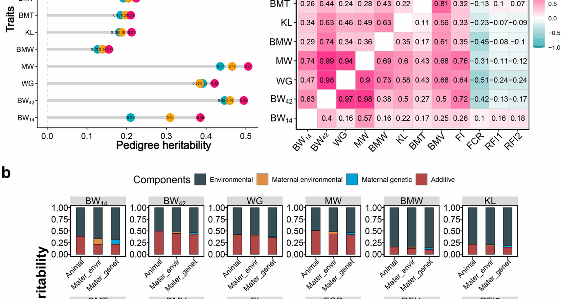
in which, \(\:\mathbf{y}\) represents the vector of phenotype value, \(\:\mathbf{X}\) is the incidence matrix of fixed effects, \(\:\varvec{\upbeta\:}\) is the vector of fixed effects of sex, batch, and season, \(\:\mathbf{Z}\) is the incidence matrix to allocate phenotypic observations to individuals, \(\:\mathbf{a}\) is the vector of additive genetic effects, and \(\:\mathbf{e}\) is the random residual effects. The \(\:\mathbf{a}\) assumed that N (0, \(\:\mathbf{A}{{\upsigma\:}}_{\text{a}}^{2}\)), where, the \(\:\mathbf{A}\) is the matrix of an additive genetic relationship constructed based on the pedigree. The heritability (\(\:{\text{h}}^{2}\)) was calculated by \(\:{{\upsigma\:}}_{\text{a}}^{2}/({{\upsigma\:}}_{\text{a}}^{2}+{{\upsigma\:}}_{\text{e}}^{2})\), in which, the \(\:{{\upsigma\:}}_{\text{e}}^{2}\) is environmental variance. There were three categories for heritability estimates: low (\(\:{\text{h}}^{2}\) \(\:{\text{h}}^{2}\) \(\:{\text{h}}^{2}\) ≥ 0.4) [28]. The strength of phenotypic and genetic correlations was classified as: little (0.0-0.2), weak (0.2–0.4), moderate (0.4–0.7), or strong (0.7-1.0) [29].
The maternal genetic effect model was listed as follows:
$$\:\mathbf{y}=\mathbf{X}\varvec{\upbeta\:}+{\mathbf{Z}}_{1}\mathbf{a}+{\mathbf{Z}}_{2}{\mathbf{m}}_{\mathbf{g}}+\mathbf{e}$$
$$\:\text{V}\text{a}\text{r}\left[\begin{array}{c}a\\\:{\text{m}}_{\text{g}}\\\:e\end{array}\right]=\left[\begin{array}{ccc}\mathbf{A}{{\upsigma\:}}_{\text{a}}^{2}&\:\mathbf{A}{{\upsigma\:}}_{\text{a}\text{m}}&\:0\\\:\mathbf{A}{{\upsigma\:}}_{\text{a}\text{m}}&\:\mathbf{A}{{\upsigma\:}}_{{\text{m}}_{\text{g}}}^{2}&\:0\\\:0&\:0&\:\mathbf{I}{{\upsigma\:}}_{\text{e}}^{2}\end{array}\right]$$
where y, X, β, \(\:\mathbf{a}\), and e were the same as terms described in the above model, and \(\:{\mathbf{m}}_{\mathbf{g}}\) was maternal genetic effect, \(\:{\mathbf{Z}}_{1}\) and \(\:{\mathbf{Z}}_{2}\) were the incidence matrix to allocate phenotypic observations to individuals and maternals, respectively. The heritability (\(\:{\text{h}}^{2}\)) was calculated by \(\:({{\upsigma\:}}_{\text{a}}^{2}+{{\upsigma\:}}_{{\text{m}}_{\text{g}}}^{2})/({{\upsigma\:}}_{\text{a}}^{2}+{{\upsigma\:}}_{{\text{m}}_{\text{g}}}^{2}+{{\upsigma\:}}_{\text{e}}^{2})\).
The maternal enviromental effect model was listed as follows:
$$\:\mathbf{y}=\mathbf{X}\varvec{\upbeta\:}+{\mathbf{Z}}_{1}\mathbf{a}+{\mathbf{Z}}_{3}{\mathbf{m}}_{\mathbf{e}}+\mathbf{e}$$
$$\:\text{V}\text{a}\text{r}\left[\begin{array}{c}a\\\:{\text{m}}_{\text{e}}\\\:e\end{array}\right]=\left[\begin{array}{ccc}\text{A}{{\upsigma\:}}_{\text{a}}^{2}&\:0&\:0\\\:0&\:{\text{I}{\upsigma\:}}_{{\text{m}}_{\text{e}}}^{2}&\:0\\\:0&\:0&\:\text{I}{{\upsigma\:}}_{\text{e}}^{2}\end{array}\right]$$
where y, X, β, \(\:\mathbf{a}\), \(\:{\mathbf{Z}}_{1}\) and e were the same as terms described in the above model, \(\:{\mathbf{m}}_{\mathbf{e}}\) was maternal permanent environmental effect, and \(\:{\mathbf{Z}}_{3}\) was the incidence matrix to allocate phenotypic observations to maternals. The heritability (\(\:{\text{h}}^{2}\)) was calculated by \(\:\left({{\upsigma\:}}_{\text{a}}^{2}\right)/({{\upsigma\:}}_{\text{a}}^{2}+{{\upsigma\:}}_{{\text{m}}_{\text{e}}}^{2}+{{\upsigma\:}}_{\text{e}}^{2})\). Genetic parameters were estimated using all 52,610 individuals from 1 to 10 generations.
Genomic prediction using GBLUP and single-step GBLUP model
The GBLUP model was presented as follows and was implemented using a linear mixed model with the ASReml-R (v4.2) software [30]:
$$\:\mathbf{y}=\mathbf{X}\varvec{\upbeta\:}+\mathbf{Z}\mathbf{a}+\mathbf{e},$$
where \(\:\mathbf{y}\), \(\:\mathbf{X}\), \(\:\varvec{\upbeta\:}\), \(\:\mathbf{a}\) and \(\:\mathbf{e}\) are the same in the BLUP animal model, while a∼N(0, G\(\:{{\upsigma\:}}_{\text{a}}^{2}\)). G was genomic relationship matrix (GRM) calculated by G = ZDZ′, where D is diagonal with \(\:{\text{D}}_{\text{i}\text{i}}=\frac{1}{\text{m}\left[2{\text{p}}_{\text{i}}\left(1-{\text{p}}_{\text{i}}\right)\right]}\) [31, 32]. In this formula, \(\:\mathbf{Z}\) is the incidence matrix of markers, \(\:{\mathbf{Z}}^{\mathbf{{\prime\:}}}\) is the transpose matrix of \(\:\mathbf{Z}\), \(\:{\text{p}}_{\text{i}}\) is the MAF at each marker. \(\:\text{m}\) is total number of markers.
In single-step GBLUP (ssGBLUP), the vector a∼N(0, H\(\:{\sigma\:}_{a}^{2}\)), where H is a combined relatedness matrix integrating both pedigree and genetic markers. The inverse of H was derived from matrices A and G using the following formula:
$$\:{\mathbf{H}}^{-1}={\mathbf{A}}^{-1}+\left[\begin{array}{cc}0&\:0\\\:0&\:{\mathbf{G}}^{-1}-{\mathbf{A}}_{22}^{-1}\end{array}\right]$$
where A22 was a numerator relationship matrix for genotyped animals using pedigree, G was a genomic relationship matrix. A was a pedigree relationship matrix from both genotyped and non-genotyped animals. This formulation facilitates the integration of pedigree and marker information into a unified framework for genetic evaluation.
Cross-validation: The data were divided into five subsets at random to conduct the cross-validation using a five-fold approach. For each subset, estimated breeding values (EBVs) were calculated using the remaining subsets as the reference population. Forward validation of G8 and G9: The 2198 individuals of G8 and G9 generations were used as the reference population, while their 296 offspring of the second hatch of G10 generation served as the validation population. The reference population of ssGBLUP included 2198 genotyped and 9223 non-genotyped ducks of G8 and G9 generations. Forward validation of G8, G9 and G10A: The 2483 individuals of G8, G9 and the first hatch of G10 generations were used as the reference population, while their 296 offspring of the second hatch of G10 generation served as the validation population. These two hatches of the G10 generation were derived from the same set of parents and were raised under the same environmental and management conditions. The reference population of ssGBLUP included 2,483 genotyped and 10,786 non-genotyped ducks of G8, G9 and the first hatch of G10 generations. Predictive accuracy was assessed by calculating the Pearson correlation coefficient between the EBVs and the corresponding adjusted phenotypic values.
Pruning markers based on LD and HWE
In a population, non-random associations of alleles at various loci are referred to as LD. More precise genetic merit prediction is possible when there is a high LD between markers and quantitative trait loci (QTL) since markers are better able to capture the genetic variance linked to selected traits [33]. We carried out the LD pruning in this study using nine thresholds of LD \(\:{\text{r}}^{2}\) (0.8, 0.6, 0.4, 0.2, 0.1, 0.075, 0.05, 0.025, 0.01). For a pair of biallelic variants (e.g., SNP1: alleles A and a; SNP2: alleles B and b) at two genomic loci. We calculated their LD \(\:{\text{r}}^{2}\) using the formula:
$$\:{\text{r}}^{2}=\frac{{({\text{p}}_{\text{A}\text{B}}-{\text{p}}_{\text{A}}{\text{p}}_{\text{B}})}^{2}}{{\text{p}}_{\text{A}}(1-{\text{p}}_{\text{A}}){\text{p}}_{\text{B}}(1-{\text{p}}_{\text{B}})}$$
where \(\:{\text{p}}_{\text{A}}\) is the frequency of allele A, and \(\:{\text{p}}_{\text{B}}\) is the allele frequency of B. \(\:{\text{p}}_{\text{A}\text{B}}\) is the frequency of haplotype AB. The LD were calculated using PLINK’s –indep-pairwise command, with a window size of 500 Kb and a step size of 50 for each \(\:{\text{r}}^{2}\) threshold [34]. GBLUP model was used to estimate EBVs. Five-fold cross-validation was used to determine the predictive accuracy for each LD threshold. To eliminate the influence of marker density on predictive accuracy, we randomly selected an equal number of variants for each LD \(\:{\text{r}}^{2}\) threshold from the original 10.3 million markers. To ensure stability, the results were averaged over 20 replicates for each LD \(\:{\text{r}}^{2}\) threshold. In the context of genomic prediction, deviations from HWE can significantly impact the accuracy of predicting genetic merit. In this study, we pruned the variants using different thresholds of HWE p-value (0.5, 0.1, 10−2, 10−4, 10−6, 10−8, 10−10, 10−13, 10−16, 10−20, 10−30, 10−40, 10−60, 10−80, 10−100, 10−150, 10−200). The HWE p-values were calculated using Chi-squared test from PLINK –hwe command [34]. We assessed predictive accuracy under these different HWE thresholds using GBLUP model. We also randomly selected an equal number of variants for each HWE thresholds from the original 10.3 million markers with 20 replicates.
Genomic predictions using bayesian models
Furthermore, we calculated the predictive accuracy of Bayesian models comprising BayesC, BayesN, BayesB, BayesR, and BayesS using LD threshold (\(\:{\text{r}}^{2}\) 7]. The Bayesian models were implemented using the GCTB software (V2.01), which employs a Gibbs sampling approach based on Markov chain Monte Carlo (MCMC) iterations [35]. Using the same fivefold cross-validation process outlined for the GBLUP model, the predictive accuracy of the Bayesian models was assessed.
Impact of prior information on genomic predictions
Integrating prior information strategically into GS frameworks is a promising method to enhance both the predictive power and practical utility of GS in breeding programs [36]. In our previous study [9], we analyzed the publicly available RNA sequencing data from seven duck tissues (adipose, muscle, liver, blood, spleen, lung, and ovary), and identified 113,374 cis-eQTLs associated with 12,266 genes. In this study, we employed the BayesRC model to incorporate prior biological information from cis-eQTLs (including their LD related variants\(\:{\:\text{r}}^{2}\) >0.1) and eGenes (variants located in eGenes and their flanking down/upstream 5 Kb regions) to enhance the prediction accuracy of GS. The Bayesian model was defined as follows:
$$\:\mathbf{y}=\mathbf{X}\varvec{\upbeta\:}+\mathbf{Z}\mathbf{s}+\mathbf{e,}$$
where \(\:\mathbf{y}\), \(\:\mathbf{X}\), \(\:\varvec{\upbeta\:}\), \(\:\mathbf{Z}\), and \(\:\mathbf{e}\) are the same as in the GBLUP model, \(\:\mathbf{s}\:\)is the sum of the vector of variant effects derived from different assumed distributions. BayesR posits that variant effects are derived from a mixture of four normal distributions, specifically N(0,\(\:\:{{\upgamma\:}}_{\text{k}}{{\upsigma\:}}_{\text{k}}^{2}\)), where the parameters \(\:\:{{\upgamma\:}}_{\text{k}}\) take values of 0, 0.01, 0.1, and 1, associated with probabilities \(\:{{\uppi\:}}_{1}\), \(\:{{\uppi\:}}_{2}\), \(\:{{\uppi\:}}_{3}\) and \(\:{{\uppi\:}}_{4}\), respectively, such that \(\:{{\uppi\:}}_{1}+{{\uppi\:}}_{2}+{{\uppi\:}}_{3}{+\:{\uppi\:}}_{4}=1\) [37]. In contrast, BayesRC is similar to BayesR but incorporates a priori independent biological information for each variant. In this model, the variant effects within functional classes are assumed to follow a mixture of the same four normal distributions with proportions (\(\:{{\uppi\:}}_{\text{f}1}\), \(\:{{\uppi\:}}_{\text{f}2}\), \(\:{{\uppi\:}}_{\text{f}3}\) and \(\:{{\uppi\:}}_{\text{f}4}\)) [38]. Meanwhile, the variant effects from variants outside of functional classes are modeled as an independent mixture of the four distributions, characterized by proportions (\(\:{{\uppi\:}}_{\text{r}1}\), \(\:{{\uppi\:}}_{\text{r}2}\), \(\:{{\uppi\:}}_{\text{r}3}\) and \(\:{{\uppi\:}}_{\text{r}4}\)).