Nonparametric baselines
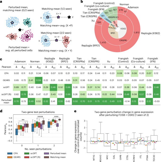
We design two nonparametric baselines that we refer to as perturbed mean and matching mean.
Perturbed mean
The perturbed mean generates a unique post-perturbation profile as the average gene expression of all perturbed cells in the train set. Let \({{\mathcal{P}}}_{{\rm{train}}}\) be the set of all perturbed cells in the train set and let xi be the gene expression of cell i. We compute the perturbed mean μpert as follows:
$${\mu }_{{\rm{pert}}}=\frac{1}{| {{\mathcal{P}}}_{{\rm{train}}}| }\sum _{i\in {{\mathcal{P}}}_{{\rm{train}}}}{{\boldsymbol{x}}}_{i}.$$
This profile is then used as a prediction for all genetic perturbations.
Matching mean
The matching mean is an extension of the perturbed mean for X+Y combinatorial perturbations. It computes post-perturbation profiles as the average of two gene expression vectors \(\mu (\,\text{X}\,)\in {{\mathbb{R}}}^{n}\) and \(\mu (\,\text{Y}\,)\in {{\mathbb{R}}}^{n}\), where n is the number of genes. Let \({{\mathcal{P}}}_{{\rm{train}}}\) be the set of all train perturbations and let \({\mathcal{P}}(\,\text{X}\,)\) be the set of cells in which gene X (or combination of genes X) was perturbed. If the single-gene perturbation X was seen at train time (X \(\in {{\mathcal{P}}}_{{\rm{train}}}\)), μ(X) corresponds to the average profile of all X-perturbed cells in the train set. Otherwise, μ(X) is equivalent to the perturbed mean μpert. Similarly, if perturbation Y was seen at train time, (Y \(\in {{\mathcal{P}}}_{{\rm{train}}}\)), μ(Y) corresponds to the average perturbation of all Y-perturbed cells in the train set. Otherwise, μ(Y) is equivalent to the perturbed mean μpert. Mathematically, we compute the matching mean μmatching(X, Y) as follows:
$$\begin{array}{l}{\mu }_{{\rm{matching}}}(\,\text{X},\text{Y}\,)=\displaystyle\frac{1}{2}\left(\;\mu (\,\text{X})+\mu (\text{Y}\,)\right),\\\qquad\qquad \mu (\,\text{X}\,)=\left\{\begin{array}{ll}\displaystyle\frac{1}{| {\mathcal{P}}(\,\text{X}\,)| }{\sum }_{i\in {\mathcal{P}}(\text{X})}{{\boldsymbol{x}}}_{i}\quad &\,\text{if}\,\,X\,\in {{\mathcal{P}}}_{{\rm{train}}}\\ {\mu }_{{\rm{pert}}}\quad &\,\text{if}\,\,X\,\notin {{\mathcal{P}}}_{{\rm{train}}}.\end{array}\right.\end{array}$$
For single-gene perturbations and combinatorial perturbations where none of the individual genes was seen at train time, the matching mean and the perturbed mean are equivalent.
Perturbation response prediction methods
We consider three perturbation response prediction methods: CPA10, GEARS1 and scGPT2 (details in Supplementary Information A).
Note about CPA
CPA was designed for predicting transcriptional responses at the single-cell level for unseen dosages and cell types. This differs from the scenario considered in this paper (generalizing across unseen genetic perturbations). It is important to emphasize that CPA does not have mechanisms to predict transcriptional responses for unseen genetic perturbations, contrary to GEARS and scGPT. At test time, we used CPA to perform counterfactual inference by sampling random control cells as input and adding the effect of the desired perturbations in the latent space.
EvaluationEvaluation setting
We consider the evaluation setting of generalization to unseen genetic perturbations, including single and combinatorial perturbations. We follow the scenario and processing steps of GEARS1, which were also adopted by scGPT2. For all datasets, we split the data by perturbation, creating a test set consisting of 25% of the genetic perturbations that are never seen during training. In the combinatorial setting, test perturbations can be divided into three groups of growing complexity: 0/2, 1/2 and 2/2 unseen genetic perturbations. We repeat this process three times using different random seeds for data splitting and model training. Thus, our results include predictions across three independent runs.
Calculating differential expression profiles
We refer to the average expression changes with respect to a population of reference cells as differential expression profiles or simply as expression changes. Mathematically, let xi be the gene expression of cell i. Let \({\mathcal{P}}(\,\text{X}\,)\) be the set of cells in which gene X (or combination of genes X) was perturbed and let \({\mathcal{C}}\) be the set of reference cells (for example, control cells). We define the differential expression profile ΔX of perturbation X as:
$${\Delta }_{{\rm{X}}}=\left(\frac{1}{| {\mathcal{P}}(\,\text{X}\,)| }\sum _{i\in {\mathcal{P}}(\,\text{X}\,)}{{\boldsymbol{x}}}_{i}\right)-\left(\frac{1}{| {\mathcal{C}}| }\sum _{i\in {\mathcal{C}}}{{\boldsymbol{x}}}_{i}\right)$$
This expression essentially computes the average transcriptional changes induced by a perturbation with respect to a population of reference cells. To estimate the average expression changes inferred by a perturbation response prediction method, we replace the first term by the average of predicted post-perturbation profiles:
$${\hat{\Delta }}_{{\rm{X}}}=\left(\frac{1}{| \hat{{\mathcal{P}}}(\,\text{X}\,)| }\sum _{i\in \hat{{\mathcal{P}}}(\,\text{X}\,)}{\hat{{\boldsymbol{x}}}}_{i}\right)-\left(\frac{1}{| {\mathcal{C}}| }\sum _{i\in {\mathcal{C}}}{{\boldsymbol{x}}}_{i}\right)$$
where \(\hat{{\mathcal{P}}}(\,\text{X}\,)\) is the set of cells for perturbation X generated by a certain method and \({\hat{{\boldsymbol{x}}}}_{i}\) is the predicted transcriptome of cell i.
Geometrically, differential expression profiles correspond to vectors in the high-dimensional gene expression space pointing to the centroid of identically perturbed cells using a specific population of cells as reference (for example, centroid of control cells). We refer to these vectors as perturbation-specific shifts.
Reference-based metrics
We refer to metrics that evaluate how well the expression changes \({\hat{\Delta }}_{{\rm{X}}}\) reflect the true expression changes ΔX as reference-based metrics. In particular, following GEARS1 and scGPT2, we used the Pearson correlation coefficient to calculate the correlation between the actual ΔX and predicted \({\hat{\Delta }}_{{\rm{X}}}\) expression changes for all held-out perturbations, using (1) all genes (PearsonΔ) and (2) the top 20 differentially expressed genes of each perturbation (PearsonΔ20). For a given perturbation X, the PearsonΔ20 scores are calculated after selecting the top 20 differentially expressed genes induced by that perturbation from both the ground truth ΔX and inferred \({\hat{\Delta }}_{{\rm{X}}}\) expression changes. Our results in Figs. 1 and 4 report the average of these scores across all held-out perturbations.
Reference-insensitive metrics
We refer to metrics that are not affected by the reference choice as reference-insensitive metrics. For example, the mean-squared error (MSE) is a reference-insensitive metric because the quantity MSE (\({\Delta }_{{\rm{X}}},{\hat{\Delta }}_{{\rm{X}}}\)) does not depend on the reference choice \({\mathcal{C}}\) (the reference cancels out). In other words, calculating the MSE on differential expression profiles ΔX and \({\hat{\Delta }}_{{\rm{X}}}\) is equivalent to calculating MSE using the post-perturbation expression profiles. In our benchmark, we employ the RMSE and calculate it using (1) all genes (RMSE) and (2) the top 20 differentially expressed genes of each perturbation (RMSE20). The RMSE20 scores are calculated after selecting the top 20 differentially expressed genes from both the ground truth and inferred post-perturbation profiles of each perturbation.
Reference-based metrics resilient to systematic variation
In Systema, we consider the same set of evaluation metrics using the average Opert of all perturbation-specific centroids O(X) as reference, which effectively emphasizes perturbation-specific effects. This centroid is computed as follows:
$${\text{O}}_{{\rm{pert}}}=\frac{1}{| {{\mathcal{P}}}_{{\rm{train}}}| }\sum _{{\rm{X}}\in {{\mathcal{P}}}_{{\rm{train}}}}\,\text{O}(\text{X}\,),\qquad \,\text{O}(\text{X}\,)=\frac{1}{| {\mathcal{P}}(\,\text{X}\,)| }\sum _{i\in {\mathcal{P}}(\,\text{X}\,)}{{\boldsymbol{x}}}_{i}$$
where \({{\mathcal{P}}}_{{\rm{train}}}\) is the set of all train perturbations, O(X) is the centroid of perturbation X and \({\mathcal{P}}(\,\text{X}\,)\) is the set of cells in which gene X (or combination of genes X) was perturbed. Our evaluation framework allows for different reference choices, including the origin, which leads to absolute post-perturbation profiles, and the average of perturbed cells.
Limitations of reference-sensitive metrics
Changing the reference to the perturbed centroid allows one to highlight perturbation-specific effects, but reference-sensitive metrics (for example, cosine similarity or Pearson correlation between perturbation-specific shifts) present some limitations. First, they might be inappropriate for evaluating weak perturbations because the norm of their shifts (with respect to the reference) is small, leading to noisy targets. That is, for weak perturbations, the presence or absence of a few single cells might have a large impact on the orientation of perturbation-specific shifts. Reference-insensitive metrics (for example, MSE) do not suffer from this limitation and have been recommended by recent studies24, but are comparatively harder to interpret. Second, reference-sensitive metrics are often invariant to perturbation strength. For example, the cosine similarity between two vectors does not depend on their norms. These metrics can thus be used to study whether methods can correctly predict the orientation of perturbation-specific shifts with respect to the reference, but not their magnitude. Finally, the reference choice can strongly influence evaluation scores and certain references may lead to undefined scores. For example, the Pearson correlation is undefined when perturbation-specific centroids overlap with the reference. In summary, reference-sensitive metrics are useful to study the relative orientations of perturbation-specific shifts and in this work we used them to investigate the extent to which perturbation response prediction methods capture systematic effects.
Centroid accuracy
To understand whether the inferred perturbation-specific centroids can accurately reconstruct the landscape of perturbations, in Systema we define a metric that we refer to as centroid accuracy. Intuitively, the centroid accuracy measures whether predicted post-perturbation profiles are closer to their correct ground-truth centroid than to the centroids of other perturbations.
Let O(X) be the centroid of perturbation X using the ground-truth expression and Opred(X) be the predicted centroid. Let \({\mathcal{P}}\) be the set of all perturbations. Mathematically, the centroid accuracy is defined as:
$$\begin{array}{l}{\rm{Centroid}}\,{\rm{accuracy}}(\,\text{X}\,)\\=\displaystyle\frac{1}{| {\mathcal{P}}| -1}\sum _{{\rm{Y}}\in {\mathcal{P}}}{\mathbb{1}}\left[d\left({\text{O}}_{{\rm{pred}}}(\,\text{X}),\text{O}(\text{X}\,)\right)
where \({\mathbb{1}}\) is the indicator function and d is a predefined distance function (we used the Euclidean distance). We calculate the centroid accuracies of test perturbations. We can similarly measure the centroid accuracy with respect to a smaller set of coarse, class-specific centroids based on available perturbation annotations (for example, perturbations inducing strong vs weak chromosomal instabilities). To do so, we simply let \({\mathcal{P}}\) be the collection of class-specific centroids, O(X) the centroid corresponding to the class assigned to X, and O(Y) the centroid of class Y.
Gene set enrichment analysis
To identify enriched pathways (between perturbed and control cells), we performed GSEA on the processed data using GSEApy30 and Biological Process 2023 gene sets from GO. We compared the populations of perturbed and control cells using signal-to-noise ratio as a ranking metric, defined as the difference of group means divided by the sum of standard deviations per group. We then ran GSEA22 with 500 random phenotype permutations (control versus perturbed) to calculate normalized enrichment scores and false discovery rates for each gene set.
AUCell
We used AUCell23 to quantify the activity of pathways in single cells. AUCell calculates the enrichment of an input gene set as the AUC across the ranking of genes in a particular cell, leading to high scores if the gene set was enriched at the top of the ranking. This allowed us to measure whether certain gene sets were consistently enriched among perturbed or control cells.
Dataset detailsData processing
We used the codebase from GEARS1 to process the data. We normalized each cell by total counts over all genes so that each cell has a total count equal to the median of total counts, followed by a log transformation. We discarded perturbations corresponding to genes not in the gene panel. This step is necessary for running scGPT (scGPT’s architecture was designed to handle perturbations of genes with available transcriptomic readouts). Following GEARS, we then selected the top 5,000 highly variable genes (HVGs) in each dataset1, and included the set of perturbed non-HVGs to the gene panel. For the Replogle15 datasets, we followed the data processing strategy of scGPT2: we retained the subset of data matching the 1,973 perturbations identified in the original study15 as inducing strong transcriptional changes, and then selected 100 cells per perturbation and 2,500 control cells. In terms of Replogle15 K562, we used the genome-wide K562 perturbation screen. In terms of the Tian16 data, we discarded the perturbations PPP4R3A (SMEK1; CRISPRa dataset) and ATP5PD (ATP5H; CRISPRi dataset) that targeted only a single cell. To process the Frangieh18 data, we followed the processing steps of Lopez et al.31 (we first converted the data from log-normalized count per millions into raw counts and removed cells with fewer than 500 expressed genes and genes expressed in fewer than 500 cells). We then selected cells perturbed with guides that exclusively target one gene. We finally normalized the data following the standard GEARS pipeline(normalize total counts, log transformation and selection of the top 5,000 HVGs plus perturbed non-HVGs) and partitioned cells into three datasets based on their condition (control, co-culture and interferon-γ). Figure 1b reflects the number of perturbations in each dataset after processing.
Control types
All datasets used non-targeting guides as controls and the Frangieh datasets18 further incorporated intergenic guides as additional controls.
Quantification of chromosomal instabilities
We downloaded the z-scored CIN annotations from Replogle et al.15. We categorized perturbations into two groups based on the extent to which they induced chromosomal instabilities: low CIN (z-score ≤ 0) and high CIN (z-score > 2).
Annotating cell cycle
To annotate cell cycle, we utilized the Scanpy32 function scanpy.tl.score_genes_cell_cycle and the cell-cycle signatures from Tirosh et al.33.
Reporting summary
Further information on research design is available in the Nature Portfolio Reporting Summary linked to this article.