Participants and samples
The studies described here comply with ethical regulations as approved under local institutional review boards, including providing written informed consent (Vanderbilt University Medical Center (VUMC) Institutional Review Board (060165 and 171657) and Western Institutional Review Board (20181836)). Peripheral PF lung samples were obtained from lungs removed at the time of lung transplant surgery at VUMC or Norton Thoracic Institute as previously described9,18,42. Control lung tissue samples were obtained from lungs declined for organ donation. Diagnoses were determined by the local treating clinicians and affiliated multidisciplinary committee and confirmed by review of explant pathology according to the current American Thoracic Society/European Respiratory Society consensus guidelines5,43. Sample names were generated based on their collection site (Vanderbilt University—‘VU’; Translational Genomics Research Institute—‘T’), disease status (healthy donor—‘HD’; interstitial lung disease—‘ILD’), unique number assigned to the patient and where applicable, whether the sample was taken from a ‘less affected’ or ‘more affected’ tissue section as determined by percent pathology scores described later in the Methods. Replicate healthy samples were labeled ‘A’ and ‘B’ to distinguish (for example, VUHD116A and VUHD116B), and replicate disease samples with the same ‘less affected’ or ‘more affected’ designation were labeled ‘1’ and ‘2’ (for example, VUILD105MA1 and VUILD105MA2).
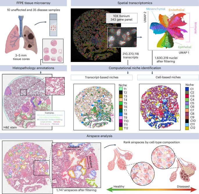
Tissue microarray (TMA) construction
To maximize efficiency per run, multiple samples could be placed on a single Xenium slide (10.45 mm × 22.45 mm) using a TMA design. A 5-µm section of each lung formalin-fixed paraffin-embedded (FFPE) block was hematoxylin and eosin (H&E) stained and presented to a physician who identified areas of interest and labeled them as less or more fibrotic (LF or MF) relative to the sample. For TMAs 1–4, blocks were designed in a 3 × 3 or 2 × 2 pattern for 3 mm and 5 mm cores, respectively (Supplementary Table 1). Sample cores were punched and placed manually using a ‘Quick-Ray Manual Tissue Microarrayer Full Set’ and ‘Quick-Ray Molds’, according to the manufacturer’s directions. Empty core spaces were filled with core punches taken from blank paraffin blocks (VWR, 76548-194). Once complete, blocks are placed face down on a clean glass slide and briefly heated in a warm drawer (~45 °C) to slightly melt the paraffin together and even the block face. TMA blocks were then cooled to room temperature, removed from the slide, sealed and stored at 4 °C.
An additional TMA was constructed (TMA5) after improvement to the 10X Xenium processing and software. TMA5 was designed in a 3 × 6 pattern of 3 mm cores with the top left core space remaining empty for orientation, with 17 samples total. A special 3 mm square tip was created by the Arizona State University Instrument Design and Fabrication Core to fit the Quick-Ray Manual Tissue Microarrayer and allow us to produce square tissue cores. Due to the new core shape, this TMA was constructed by placing each core individually on double-sided adhesive tape (Gorilla Double-Sided Mounting Tape) in a paraffin block mold44. The entire mold is warmed to 37 °C, and a P1000 is used to dispense 400 μl of melted paraffin wax in the lanes between the cores. As more wax was poured into the back of the mold, the mold was gently tapped to dislodge air bubbles. Once solidified, the block was extracted from the mold, and the tape was removed. TMA5 then underwent the same warm drawer and storage conditions as all others.
During TMA preparation, some samples were placed closely together such that a subset of transcripts and nuclei could not be distinguished as belonging specifically to either sample. These transcripts and nuclei were removed from downstream analyses.
All samples were processed through the Xenium workflow, and four specific samples from TMA5 (one unaffected and three PF) were then additionally run through the Visium HD protocol after Xenium processing to generate orthogonal data for verifying phenomena of interest. Both workflows are described below.
Xenium in situ workflowGene panel design
Xenium in situ technology requires the use of a predefined gene panel. Each probe contains two paired sequences complementary to the targeted mRNA as well as a gene-specific barcode. Upon binding of the paired ends, ligation occurs. The now circular probe is amplified via rolling circle amplification, increasing the signal-to-noise ratio for target detection and decoding. A total of 343 unique genes were included in the analysis of this dataset. A total of 246 genes came from an early version of the Xenium human lung base panel (PD_277) and 97 genes from a custom-designed panel (CVEVZD). The custom panel was curated based on human lung single-cell analysis data18, selecting genes useful for cell-type identification and/or suspected to be involved in IPF.
Xenium sample preparation
As Xenium in situ technology examines RNA, all protocol workstations and equipment were cleaned using RNase AWAY (RPI, 147002) followed by 70% isopropanol. All reagents, including water, were molecular-grade nuclease-free. Sample preparation began with rehydrating and sectioning FFPE blocks on a microtome (Leica, RM2135). Sections measuring 5 µm were placed onto Xenium slides (10X Genomics). Following overnight drying, slides with placed samples were stored in a sealed desiccator at room temperature for ≤10 days. Slides were then placed in imaging cassettes for the remainder of the preparation. Tissue deparaffinization and decross-linking steps made subcellular RNA targets accessible. Gene panel probe hybridization occurred overnight for 18 h at 50 °C (Bio-Rad DNA Engine Tetrad 2). Subsequent washes the next day removed unbound probes. Ligase was added to circularize the paired ends of bound probes (2 h at 37 °C) and followed by enzymatic rolling circle amplification (2 h at 30 °C). TMA5 was prepped to include Xenium Multi-Tissue Stain (10X Genomics, 1000662) according to 10X Genomics’ Demonstrated Protocol CG000749. All slides were washed in Tris-EDTA (TE) buffer before background fluorescence was chemically quenched; autofluorescence is a known issue in lung tissue as well as a byproduct of formalin fixation45. Following PBS and PBS-T washes, DAPI was used to stain sample nuclei. Finalized slides were stored in PBS-T in the dark at 4 °C for ≤5 days until being loaded onto the Xenium Analyzer instrument. Stepwise Xenium FFPE preparation guidelines and buffer recipes can be found in 10X Genomics’ Demonstrated Protocols CG000578 and CG000580.
Xenium Analyzer instrument
The Xenium Analyzer is a fully automated instrument for decoding subcellular localization of RNA targets. The user marks regions for analysis by manually selecting the sample location on an initial low-resolution, full-slide image. After loading consumable reagents and a maximum of two slides per run, internal sample and liquid handling mechanics control experiment progression. Data collection occurs in cycles of fluorescently labeled probe binding, image acquisition and probe stripping. Images of the fluorescent probes are taken in 4,240 × 2,960-pixel fields of view (FOVs). Localized points of fluorescence intensity detected during the rounds of imaging are then defined as potential RNA puncta. Each gene on the panel has a unique fluorescence pattern across the image channels. Puncta that match a specific pattern is then decoded and labeled according to the gene ID. Finally, all image FOVs and associated detected transcripts are computationally stitched together via the DAPI-stained image. Onboard analysis pipelines present quality values for each detected transcript, based on variable confidence in the signal and decoding process. Data for TMA1–TMA4 were acquired on instrument software version 1.1.2.4 and analysis version xenium-1.1.0.2. Data for TMA5 were acquired on instrument software version 2.0.1.0 and analysis version xenium-2.0.0.10. TMA5 had additional fluorescent images taken of each Xenium Multi-Tissue Stain channel to allow for cell segmentation. Detailed instructions on instrument operation and consumable preparation can be found in 10X Genomics’ Demonstrated Protocol CG000582.
Postrun histology
After the run, slides were removed from the Xenium Analyzer instrument and had quencher removed according to 10X Genomics’ Demonstrated Protocol CG000613. Immediately following, the slides were H&E stained according to the following protocol: xylene (x3, 3 min ea), 100% alcohol (x2, 2 min ea), 95% alcohol (x2, 2 min ea), 70% alcohol (2 min), deionized (DI) water rinse (1 min), hematoxylin (1 min; Biocare Medical CATHE), DI water rinse (1 min), bluing solution (1 min; Biocare Medical HTBLU-M), DI water rinse (3 min), 95% alcohol (30 s), eosin (5 s; Biocare Medical HTE-GL), 95% alcohol (10 s), 100% alcohol (x2, 10 s ea) and xylene (x2, 10 s ea). Coverslipping was performed using Micromount (Leica, 3801731) and cured overnight at room temperature. Histology images were taken on a ×20 Leica Biosystems Aperio CS2.
Data preprocessingCell segmentation
Cell segmentation was performed with 10X Xenium onboard cell segmentation (10X Genomics). DAPI-stained nuclei from the DAPI morphology image were segmented, and boundaries were consolidated to form nonoverlapping objects. For samples on TMAs 1–4, nuclear boundaries were expanded by 15 µm or until they reached another cell boundary to approximate cell segmentation. For samples on TMA5, cells were segmented using a cell boundary stain. For all TMAs, nuclear segmentation was used to define cells.
Image registration
Registration was performed between Xenium DAPI morphology images (that is, nuclei) and H&E-stained images of the same slice with the BigWarp plugin implemented in ImageJ (2.14.0)46,47. To place both images in the coordinate space of the DAPI morphology image, the H&E stained image was specified as the moving image, and the DAPI morphology was specified as the target. Anchors were placed on identifiable landmarks on both images (approximately 200 landmarks per image pair). A thin plate spline warp was then applied to align the corresponding anchor points between the two images. Registered images were manually reviewed for potential visual artifacts resulting from the registration process. These registered images were then visualized in Xenium Explorer 3.0.0 software, which was used to generate figures showing transcript expression overlain on H&E stains.
Quality filtering and data preprocessing
For each sample, Xenium generated an output file of transcript information, including x and y coordinates, corresponding gene, assigned cell and/or nucleus and quality score. Low-quality transcripts (quality value (QV) 32. Nucleus-by-gene count matrices were created for each sample based on the expression of transcripts that fell within segmented nuclei. A single merged Seurat object was created for all samples based on these count matrices and metadata files with nuclei coordinates and area. Nuclei were retained according to the following criteria: ≥12 transcripts corresponding to ≥10 unique genes, percentage of high-quality transcripts corresponding to negative control probes, negative control codewords, unassigned codewords, or the cumulative percentage of these ≤5, and nucleus area ≥6 and ≤80 µm. Because Xenium outputs coordinates based on each slide, which results in samples with shared coordinates across multiple slides, the nuclei coordinates were manually adjusted for visualization so that no samples overlapped during plotting. These adjusted nucleus coordinates were added to the Seurat object as a dimension-reduction object.
Dimensionality reduction, clustering and cell-type annotation
Scanpy48 in Python was used to perform dimensionality reduction and clustering, while Seurat v5 (ref. 32) in R was used for visualization of these results49. Gene expression was normalized per cell using a log1p transformation. Dimensionality reduction was performed with principal component analysis. Nuclei were clustered using the Leiden algorithm50 based on this dimensionality reduction and computing a nearest neighbors distance matrix. Uniform Manifold Approximation and Projection (UMAP) plots of the data were then generated for visualization. For speed, these calculations were performed using a container51 with the RAPIDS (v21.8.1) implementation52 of Scanpy (v1.8.1).
For cell-type annotation, we used both marker genes and spatial information. We did not rely solely on gene expression because some level of gene ‘contamination’ is expected with spatial data, as transcripts located in one cell may be assigned to an adjacent cell in sufficiently close proximity. Therefore, we incorporated spatial data including cell morphology and histological features to label clusters. Initial Leiden clusters were primarily segregated by cell lineage based on marker genes assessed using the Seurat v5’s FindMarkers function, including PECAM1 (endothelial), EPCAM (epithelial), PTPRC (immune), DCN, LUM and COL1A1 (all mesenchymal)32. New Seurat/AnnData objects were created for each of the four lineages, and dimensionality reduction and clustering were performed again as described above. Clusters were then given first-pass cell-type labels based on marker genes. The epithelial and immune lineages were further split into sublineages for alveolar and airway cells (epithelial) as well as myeloid and lymphoid cells (immune), and new Seurat/AnnData objects were generated and reprocessed for these sublineages. As lineage and subgroup splitting became more accurate, clusters were relabeled with revised annotations. ‘Stray’ clusters that did not belong to the lineage or sublineage they were originally assigned to, as well as clusters that were marked by genes from more than one lineage, received final annotations based on shared marker genes and spatial patterns with confidently labeled clusters. Low-quality clusters with extremely low transcript counts and/or with conflicting marker genes that could not be resolved (similar to ‘doublets’ in scRNA-seq data) were removed. This resulted in 47 final cell types, including 4 endothelial, 12 epithelial, 22 immune and 9 mesenchymal (Extended Data Figs. 2–5 and Supplementary Table 2).
H&E image annotationPercent pathology assignment
Percent pathology was assessed by visual estimation of the fraction of the total imaged area of the sample with architectural remodeling. Disease samples were labeled ‘more affected’ if their percent pathology was greater than or equal to 75%. All other disease samples were labeled ‘less affected’, and control samples were labeled ‘unaffected’ regardless of percent pathology score.
Annotation of histological features
We annotated representative examples of 27 histological features across all 45 samples, including 12 epithelial or of likely epithelial origin (normal alveoli, minimally remodeled alveoli, hyperplastic AECs, emphysema, remodeled epithelium, advanced remodeling, epithelial detachment, remnant alveoli, small airway, large airway, microscopic honeycombing and goblet cell metaplasia), 3 vascular (artery, muscularized artery and venule), 3 immune (granuloma, mixed inflammation and TLS), 5 mesenchymal/interstitial (interlobular septum, airway smooth muscle, fibroblastic focus, fibrosis and severe fibrosis) and 2 general (multinucleated cell and giant cell) feature types. Annotations were marked on the registered H&E images using QuPath (v.0.4.3)53. Cells were then assigned to annotated regions using a custom Python (v.3.12.3) script. Briefly, annotated regions were scaled by a factor of 0.2125 µm per pixel to harmonize units with the cell centroid coordinates. Cells were assigned a boolean value for each annotated region corresponding to whether the cell centroid fell within the annotated region. After filtering to annotations containing at least one cell, there were 712 annotations across the 27 histological features.
Comparison to scRNA-seq datasets
We compared cell lineage recovery from the present spatial dataset to two scRNA-seq sources. The first was ref. 9, a recent sc-eQTL study from our lab9, and the other was the Human Lung Cell Atlas (HLCA), which included aggregated data from multiple lung scRNA-seq studies12. Studies from the HLCA varied in the disease studied and whether the dataset contained control and/or lung disease samples. We narrowed the scope of our comparison to studies (lung atlases) or samples (sc-eQTL study) that did not specifically enrich or deplete cells from a specific lineage in their preprocessing and did not exclusively contain data from nasal samples. We included 47 samples from the sc-eQTL study (19 control and 28 ILD) and 14 datasets from the HLCA. For each data source, the proportion of cells from each lineage (endothelial, epithelial, immune and mesenchymal) was calculated first for all samples and then for control and disease samples separately. If an annotated cell type did not have a clear lineage association, it was removed from the analysis. Sample-level data from the present study was compared to sample-level data from the sc-eQTL study and dataset-level information from HLCA.
Post-Xenium Visium HD workflow for select samplesPost-Xenium Visium HD sample preparation
All protocol workstations and equipment were cleaned using RNase Away (RPI 147002) followed by 70% isopropanol. All reagents, including water, were molecular-grade nuclease-free. The Xenium slide containing IPFTMA5 was H&E stained postrun as described in ‘Xenium in situ workflow—Postrun histology’. The slide was stored for 9 days postcoverslipping in a sealed desiccator at 4 °C. The slide was then decoverslipped in xylene, loaded into a Visium tissue slide cassette (10X Genomics), and destained using 0.1 N HCl. The decross-linking step of the archived slide protocol was skipped due to this already being performed as part of the Xenium workflow. Stepwise archived slide preparation guidelines and buffer recipes can be found in 10X Genomics’ Demonstrated Protocol CG000684.
Visium HD CytAssist preparation
The tissue slide within the Visium HD tissue cassette was then prepared for loading onto the CytAssist instrument. It underwent human probe hybridization (10X Genomics, 1000466) and a posthybridization wash to remove unbound probes, followed by probe ligation and subsequent wash. The Visium HD slide containing the probe capture areas was prepared. Both the Visium HD slide and the tissue slide were loaded onto the CytAssist instrument to enable the probe release and capture. Four samples were targeted as a representative subset (one unaffected and three fibrotic) for the Visium HD analysis (VUHD049, VUILD49LA, TILD111LA and TILD113LA) as it has a smaller capture area than the Xenium slide. Once captured on the Visium HD slide, probes were extended, eluted into 0.08 M KOH and then transferred into 1 M Tris–HCl (pH 8). Pre-amplification cleanup was performed using SPRIselect reagent (Beckman Coulter, B23318). The sample was stored at 4 °C overnight. Detailed instructions regarding Visium HD CytAssist operation, tissue cassette and Visium HD slide preparation can be found in 10X Genomics’ Demonstrated Protocol CG000685.
Visium HD library construction and sequencing
The probe-based library was constructed using Dual Index Plate TS Set A (10X Genomics, 1000251) with a sample index PCR cycle number of 16, as determined by the Cq value from qPCR (Applied Biosystems QuantStudio 5). A final cleanup step with SPRIselect reagent was followed by storage at −20 °C until sequencing. Library quality control was performed on an Agilent TapeStation 4200. Next-generation sequencing was carried out on Illumina’s NovaSeq X platform using a 10 billion read, 300 cycle flow cell. Minimum sequencing recommendations were met using the product of tissue coverage percentage estimations and a constant maximum read figure of 275 million read pairs. Optimal cluster density was achieved with a lane loading concentration of 235 pM. All steps were performed according to the instructions found in 10X Genomics’ Demonstrated Protocol CG000685.
Visium HD data processing
A high-resolution image was aligned using the Visium HD Manual Alignment tool on Loupe Browser (v8.0.0; 10X Genomics)54. Five matched landmarks per sample within the capture area were selected for the alignment and then algorithmically refined by the software. Visium HD sequence data, high-resolution image and alignment file were processed using the count function of Spaceranger (3.0.0; 10X Genomics)55 with default parameters. Reads were mapped against the GRCh38-2020-A reference.
Visium HD data analysis
To compare the Xenium and Visium HD outputs, the Loupe Browser (v8.0.0) software was used to visualize gene expression over H&E images for the Visium HD data. Composite gene expression scores were used to visualize marker gene expression of several cell types of interest. These composite scores were created by summing the log2-transformed unique molecular identifier (UMI) counts of 7–26 genes per cell type that were selected based on the dotplot heatmap in Extended Data Fig. 1 and prior literature (KRT5−/KRT17+ ‘aberrant basaloid’ cells18,19; activated fibrotic fibroblasts56; alveolar FABP4+ macrophages24,37; SPP1+ macrophages24,37; Supplementary Table 10). Three strong canonical marker genes for KRT5−/KRT17+ cells or activated fibroblasts (COL1A1, FN1 and ACTA2) were not included in the composite scores for these cell types because they mark both cell types (COL1A1 and FN1) or because they strongly mark another cell type (ACTA2 marks smooth muscle). For the comparison between alveolar macrophages and SPP1+ macrophages (Fig. 6h), genes that were strong markers for both macrophage populations in the present Xenium dataset according to Supplementary Figs. 3 and 6 were excluded from the alveolar macrophage marker list, except for PPARG, which is known to distinguish these populations in scRNA-seq and had low expression in SPP1+ regions in the Visium HD data.
Computational niche identificationTranscript-based niches
Transcript-based niches were characterized using a graph neural network model GraphSAGE (implementation in StellarGraph v1.2.1 + Python 3.8.0)31,57 that directly modeled detected transcripts without cell segmentation. GraphSAGE learns the structures in the graph data via sampling and aggregating neighbors, scaling well to large graphs. Detected transcripts from each sample were used to build a sample graph after removing low-quality transcripts (QV) d = 3.0) similar to a previous study57. Each node was associated with an input feature vector that was the one-hot encoding of the node’s gene label, and small components with nodes with fewer than ten nodes were removed (n = 299,018,086 after filtering).
A two-hop GraphSAGE model was applied to learn node embeddings. It sampled 20 and 10 neighboring nodes at the first-hop and second-hop neighbors, respectively, to learn 50-dimensional embeddings at each hop for each node in the graph. To embed all nodes across samples into the same embedding space, we trained the model on a joined graph consisting of subgraphs from 28 samples (TMAs 1–4) with each subgraph containing 5,000 randomly sampled root nodes along with their three-hop neighbors as well as the existing edges among them. The joined graph contained 18,594,542 nodes and 421,316,086 edges for model training. The model was trained in an unsupervised manner by solving a binary classification task for ‘positive’ and ‘negative’ node pairs, in which the model predicts whether or not two nodes should have an edge connection based on their local neighborhood structures. We trained the model with ten epochs, achieving a training accuracy of 0.82 (ref. 31).
Embedding representations of all nodes (transcripts) across the 28 samples from TMAs 1–4 were obtained using the trained model, and we performed unsupervised clustering on all nodes using the Gaussian mixture model (k = 12) as implemented in the PyCave library (https://github.com/borchero/pycave). We subsequently obtained the embeddings of the 17 samples from TMA5 using the same trained model and projected their transcripts into the existing 12 transcript clusters.
Transcript-based niche plots and assignment of nuclei to niches
We created a hexbin summarization plot for each sample using all transcripts with a bin width of 5 for generating the transcript-based niche plots to overcome overplotting issues. Each bin was labeled and colored with the major cluster label among the transcripts falling in the bin area. Bins with fewer than ten transcripts were not included in the plots. To assign cells to transcript-based niches, we assigned each cell to its closest hexbin by calculating the Euclidean distance of each cell centroid to the hexbin centroids.
Cell-based niches
Seurat v5’s32 BuildNicheAssay function was used to partition cells into 12 spatial niches using k-means clustering based on the cell-type composition of their 25 closest neighboring cells.
Cell-type proximity analysis
To assess proximity between cell types, each cell was anchored, and its distance and angular direction were calculated between the anchored cells and their neighboring cells within a fixed 60-µm radius circle. Only first-degree neighbors were considered proximal to the anchored cell. The probability of cell types being proximal to one another was assessed using logistic regression by assigning cells to binarized proximal and nonproximal categories and using cell type as a covariate. This analysis was performed both for all samples and cell types and within each cell and transcript niche individually.
Differential expression and composition analysesDifferential cell-type composition by disease severity
We transformed the cell-type proportion per sample using logit transformation and tested whether the cell-type proportion was different among three disease groups (unaffected, less affected and more affected samples) using the propeller.anova function implemented in propeller58.
Representative gene detection in transcript-based niches
We used the linear model framework implemented in propeller58 and limma59,60 to test differences in gene proportions across niches and thereby identify representative genes of each niche. We first investigated the proportion of transcripts assigned to each niche within each sample. Samples were excluded from testing for a niche when a few transcripts from that sample (proportion −4) were assigned to the niche. Gene proportions were logit-transformed, and a linear model was fitted to each gene that modeled the mean transformed gene proportion in each niche while accounting for sample differences. Differentially abundant genes were then derived by contrasting the mean gene proportion from one niche with the average mean proportion from the other niches.
Differential expression, cell-type composition and niche proportions by percent pathology
We used the same propeller58 and limma59,60 frameworks for finding gene, cell type and niche proportions that correlated with changes in percent pathology across samples. Proportions were logit-transformed, and linear models were fit to model the relationship between the transformed proportions and percent pathology across samples to find features (that is, genes, cell types and niches) that varied significantly with percent pathology (FDR
We also performed a cell-type-aware differential gene expression along percent pathology across samples by pseudo-bulking gene expression per identified cell type. For each cell type, we filtered the list of testing genes to remove contamination signals. To identify contamination genes per cell type, we first scaled the gene counts using a count-per-1K normalization across cells and kept genes with at least five counts in 30% of cells within a cell type for testing. The remaining genes per cell type were then tested with the propeller58 and limma59,60 frameworks.
Differential expression analysis across annotated pathology features
We aggregated gene counts from cells included in each pathology annotation instance and detected differentially expressed genes among pathology annotations by fitting linear models implemented in limma59,61. Gene expression was converted to counts per million (CPM) and log2-transformed after adding a 0.5 pseudocount. Lowly expressed genes (log2(CPM) 2CPM observation value, which was subsequently used in the linear regression model to account for heteroskedasticity in count data. We controlled for the TMA effects by adding TMA origins as a covariate in the linear model. Differentially expressed genes for each annotation type were detected by comparing the gene expression per annotation type with the rest. Separately, we also compared epithelial annotations to each other to identify dysregulated genes in pathologic epithelium.
Lumen segmentation and airspace identificationInitial lumen segmentation
To segment individual lumens from the spatial sequencing data, a custom graphics processing unit (GPU)-accelerated image processing algorithm was developed using scikit-image (v.0.19.3), RAPIDS cuCIM (v.22.12.00) and CuPy (v.11.2.0) in Python (v.3.9.7) to assign unique identifiers to lumens in the spatial transcriptome data62,63,64. Briefly, the location of each detected transcript, excluding transcripts associated with immune cells, was binarized to a 2D image followed by a series of dilation, erosion and closing operations to define the location of the tissue and segment the lumens. The outer boundaries of the tissue were defined using Alpha Shapes (alphashape package v.1.3.1) on a denoised, closed shape representing the entire tissue. Unique identifiers were then assigned to the negative space (lumens) using scikit-image, and metrics were calculated for each individual lumen. Cell centers (nuclei) within a cutoff distance, defined as the thickness of a normal alveolar wall, were then assigned to the unique identifier of the closest lumen by searching for the nearest label in a restricted zone using the K-D Tree nearest-neighbor lookup algorithm implemented in scikit-image. All cells that were not close to a lumen were given an identifier of zero.
Quality filtering to isolate alveolar airspaces
Lumens were first filtered by size to remove false positive segmentations. We retained lumens that contained between 25 and 500 cells, including at least 5% epithelial cells, for which the maximum distance between any two nuclei in the lumen was at least 110 µm. The high cell number and low epithelial cell thresholds were selected to retain lumens with large macrophage accumulations. For each lumen, the proportion of cells belonging to each cell niche was calculated, and the cell niche(s) with the highest proportion of cells was recorded as the ‘maximum cell niche’. To discard lumens corresponding to endothelial and airway structures, lumens were required to have an endothelial niche proportion of C10 KRT5−/KRT17+ fibrotic niche) and/or C11 (airspace macrophage accumulation niche).
Assessing changes in cell types, niches and gene expression along pseudotime
Pseudotime analysis was performed on the remaining 1,747 alveolar airspaces based on the proportion of transcripts overlapping nuclei that were assigned to the T4 healthy alveolar niche. This allowed us to rank airspaces along a continuum of disease severity and tissue remodeling. To find cell types, niches and genes with varied abundances or expression along the pseudotime, we applied GAMs using the fitGAM function from tradeSeq65 on the aggregated feature counts across airspaces under a negative binomial distribution. We subsequently applied associationTest65 to test the association of features with pseudotime.
Cell-type changes along pseudotime-ordered airspaces
We counted the number of each cell type across airspaces and fitted a GAM model per cell type against pseudotime with an offset of log-transformed total cell counts. We excluded cell types if they were not present with at least three counts in at least ten airspaces (36 cell types tested). We obtained the list of significant cell types (28 in total) using the associationTest65.
Cell-type-based and transcript-based niches
We applied similar analysis for cell-type-based and transcript-based niches as for cell-type analysis given above. Niches were excluded if they were not present with at least three counts in at least 10% of segmented airspaces. We obtained the smoothed niche abundance changes along 2,000 time points after model fitting and visualized their patterns in heatmaps after ordering them by their peak time point. The peak time point for each niche was determined using a rolling mean approach (window size, n = 100). Features with earlier peak times were plotted in the top rows.
Classifying gene expression patterns along pseudotime
We characterized gene expression patterns along pseudotime-ordered airspaces using GAM models by modeling the gene count along pseudotime under negative binomial distribution. We added the total number of detected transcripts per lumen as an offset term as well as a TMA covariate for controlling TMA effects. With the fitted model, we predicted the gene expression along pseudotime and clustered the gene expression patterns first using hierarchical clustering (k = 20) after taking z scores per gene. Genes were separated into bimodal and unimodal patterns by visual inspection of the 20 hierarchical clusters. For the unimodal genes, we further clustered them by spectral clustering (k = 4) using the R package kernlab66. We ordered the four gene clusters by their gene expression peak times and labeled them into four categories, including homeostasis, early remodeling, intermediate remodeling and late remodeling. The gene expression dynamics of the four gene clusters were then visualized in heatmaps.
Altered gene expression along pseudotime within each cell type
We tested which genes had altered expression along pseudotime within a specific cell type using GAMs as well. We tested 25 cell types that were observed with more than three cells in at least 80 airspaces. For each cell type, we aggregated their gene expression across segmented airspaces. Within a specific cell type, for the expression of each gene \(\mu\), we fit a negative binomial GAM model to model the gene expression across lumens using the gam function with cubic regression splines ‘bs=“cr”’ implemented in mgcv67 as
$$\log (\mu )=s(t)+\mathop{\sum }\limits_{i=1}^{15}s({p}_{i})+\,\log (n)+U,$$
where t represents pseudotime, pi represents the proportion of cell type i, n represents the number of total transcripts per lumen and U represents the TMAs. We applied the same strategies in knot selection as in tradeSeq65 and selected five knots per smooth term. We included proportions of 15 major cell types that had more than three cells in more than 300 airspaces in the model to control for the contamination in detected gene expression signals. When testing genes for significant association with pseudotime per cell type, we restricted genes to the set of significant genes in the overall gene association test across all cell types. For each cell type, we then tested genes that were detected with more than three copies in 50% of the testing airspaces. Genes that had significant pseudotime terms after multiple testing corrections (FDR
Statistics and reproducibility
Sample sizes were chosen based on sample availability, although data generation was randomized with respect to disease and control samples. The study was unblinded. Any data exclusions are noted above, including filtering cells of a large size or unexpectedly low or high gene counts based on current best practices. Key findings from Xenium data were replicated with orthogonal technology (Visium HD) as described above. For figures depicting H&E images of described phenomena (for example, cell types in annotations in Fig. 3d and macrophage accumulations in Fig. 6c–e,g–h), at least three similar examples were observed across samples, and the images shown are intended to be representative but not exhaustive. For representative H&E images overlain with transcripts or cell types, see the accompanying dotplot heatmaps for additional context. Full data are available at the Gene Expression Omnibus (GEO), including histopathology, gene expression data and cell-type annotations.
Reporting summary
Further information on research design is available in the Nature Portfolio Reporting Summary linked to this article.